InputOutputResponse
InputOutputResponse[sys,u,tspec]
入力信号 u,一次指定 tspec で入出力モデル sys の応答を与える.
InputOutputResponse[sys,…,"prop"]
特性"prop"の値を与える.
詳細とオプション
- InputOutputResponse は,シミュレーションとしても知られている.
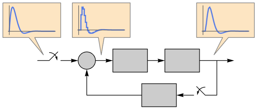
- InputOutputResponseは,しばしば,プラントとコントローラのような系全体のシミュレーションを行い,系の動作を正確に分析し,パフォーマンスを検証し,コントローラ努力を測定するために使われる.
- 結果は,sys のもとになっている方程式を解くことで計算される.一般的には,混合連続または離散系についての,常微分方程式または常差分方程式あるいはそれらの組合せである.
- 混合連続/離散時間系については,結果は連続時間であるが値が区分的であることが多い.
- SystemsConnectionsModelとして表される系については,内部信号もすべて計算することができる.
- 入出力モデルl sys は以下の形を取ることができる.
-
TransferFunctionModel[…] 伝達関数モデル StateSpaceModel[…] 状態空間モデル AffineStateSpaceModel[…] アフィン状態空間モデル NonlinearStateSpaceModel[…] 非線形状態空間モデル DiscreteInputOutputModel[…] 離散入出力モデル SamplerModel[…] サンプル採取器モデル HolderModel[…] ホールダーモデル SystemsConnectionsModel[…] 接続モデル - InputOutputResponse[{sys,ics},…]を使って初期条件 ics が指定できる.
- 入力信号 u は以下の形を取ることができる.
-
{u1[t],…,up[t]} 時間 t の関数としての連続時間信号 ui[t] {{u11,…,u1k},…,{up1,…,upk}} 離散時間信号のシーケンス{ui1,…,uik} {…,ui[t],…,{uj1,…,ujk},…} 連続時間信号と離散時間信号の組合せ - 一次指定 tspec は以下の形を取ることができる.
-
t  の関数としての記号解を計算する
{t,0,tmax} 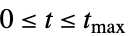 のときの数値解または記号解を計算する
 - 特性"prop"は以下の形を取ることができる.
-
"Data" InputOutputResponseDataオブジェクト "OutputResponse" リストとしての出力応答 "OutputResponseAssociation" 連想としての出力応答 "PropertyAssociation" 連想としての特性名と値 "PropertyDataset" Datasetとしての特性名と値 "StateResponse" リストとしての状態応答 "StateResponseAssociation" 連想としての状態応答 "SubsystemOutputResponse" リストとしての部分系の出力応答 "SubsystemOutputResponseAssociation" 連想としての部分系の出力応答 {p1,p2,…} 特性 piの値 - InputOutputResponseは,以下の値を取るMethodオプションを取る.
-
"DSolve" DSolve "Integrate" Integrate "Iterate" 積分して解を得る "NDSolve" NDSolve "RecurrenceTable" RecurrenceTable "RSolve" RSolve "Sum" Sum - Method{m,opt1val1,…}のメソッド m は,オプション optiを値 valiに設定して用いられる.
例題
すべて開く すべて閉じる例 (4)
InputOutputResponse[TransferFunctionModel[{{{ω^2}}, s^2 +
2*s*ζ*ω + ω^2}, s], 1, t]//SimplifyStateSpaceModel[m x''[t] + c x'[t] + k[t] == f[t], x[t], f[t], x[t], t];
InputOutputResponse[%, DiracDelta[t], t]InputOutputResponse[SystemsConnectionsModel[{TransferFunctionModel[{{{s}}, 1 + s}, s],
TransferFunctionModel[{{{1}}, 1 + s + s^2}, s], TransferFunctionModel[{{{1, 1}}, 1}, s],
TransferFunctionModel[{{{1}}, 1 + 0.1*s + s^2}, s]}, {{1, 1} -> {3, 1}, {2, 1} -> {3, 2},
{3, 1} -> {4, 1}}, {{1, 1}, {2, 1}}, {{4, 1}}], {-1, 3}, {t, 0, 100}]Plot[%, {t, 0, 100}, PlotRange -> All]ℛ = InputOutputResponse[SystemsConnectionsModel[{TransferFunctionModel[{{{s}}, 1 + s}, s],
TransferFunctionModel[{{{1}}, 1 + s + s^2}, s], TransferFunctionModel[{{{1, 1}}, 1}, s],
TransferFunctionModel[{{{1}}, 1 + 0.1*s + s^2}, s]}, {{1, 1} -> {3, 1}, {2, 1} -> {3, 2},
{3, 1} -> {4, 1}}, {{1, 1}, {2, 1}}, {{4, 1}}], {-1, 3}, {t, 0, 100}, "Data"]ℛ["OutputResponse"]ℛ["SubsystemOutputResponse"]ℛ["Properties"]スコープ (31)
基本的な用法 (9)
InputOutputResponse[TransferFunctionModel[{{{1}}, 1 + s}, s], UnitStep[t], {t, 0, 10}]Plot[%, {t, 0, 10}, PlotRange -> All]InputOutputResponse[TransferFunctionModel[{{{1}}, 1 + s}, s], UnitStep[t], t]//SimplifyPlot[%, {t, 0, 10}, PlotRange -> All]InputOutputResponse[StateSpaceModel[{{{0, 1}, {-1, -5}}, {{0}, {1}}, {{1, 0}}, {{0}}}, SamplingPeriod -> None,
SystemsModelLabels -> None], UnitStep[t], t]//SimplifyPlot[%, {t, 0, 30}, PlotRange -> All]InputOutputResponse[StateSpaceModel[{{{0, 1}, {-1, -5}}, {{0}, {1}}, {{1, 0}}, {{0}}}, SamplingPeriod -> None,
SystemsModelLabels -> None], UnitStep[t], t, "StateResponse"]//SimplifyPlot[%, {t, 0, 30}, PlotRange -> All]InputOutputResponse[{StateSpaceModel[{{{0, 1}, {-1, -5}}, {{0}, {1}}, {{1, 0}}, {{0}}}, SamplingPeriod -> None,
SystemsModelLabels -> None], {2, 3}}, UnitStep[t], t, "StateResponse"]//Simplify% /. t -> 0InputOutputResponse[StateSpaceModel[{{{0, 1, 0}, {-2, -3, 0}, {0, 0, -1}}, {{0, 0}, {1, 0}, {0, 1}}, {{0, 1, 1}},
{{0, 0}}}, SamplingPeriod -> None, SystemsModelLabels -> None], {UnitStep[t], Sin[t]}, t]より少ない信号しか指定されていなければ,残りの入力にはデフォルト値(通常は0)が選ばれる:
With[{ssm = StateSpaceModel[{{{0, 1, 0}, {-2, -3, 0}, {0, 0, -1}}, {{0, 0}, {1, 0}, {0, 1}}, {{0, 1, 1}},
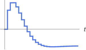
{{0, 0}}}, SamplingPeriod -> None, SystemsModelLabels -> None]}, InputOutputResponse[ssm, UnitStep[t], t] == InputOutputResponse[ssm, {UnitStep[t], 0}, t]]InputOutputResponse[StateSpaceModel[{{{-0.5}}, {{1}}, {{0.5}}, {{0}}}, SamplingPeriod -> 1, SystemsModelLabels -> None], Table[1, 10]]ListStepPlot[%, DataRange -> {0, 9}]InputOutputResponse[StateSpaceModel[{{{-0.5}}, {{1}}, {{0.5}}, {{0}}}, SamplingPeriod -> 1, SystemsModelLabels -> None], 1, {t, 0, 9}]入力シーケンスは,系のサンプリング周期を考慮して生成される:
InputOutputResponse[StateSpaceModel[{{{-0.5}}, {{1}}, {{0.5}}, {{0}}}, SamplingPeriod -> 0.25], Sin[t], {t, 0, 5}]InputOutputResponse[StateSpaceModel[{{{-0.5}}, {{1}}, {{0.5}}, {{0}}}, SamplingPeriod -> 0.25], Table[Sin[t], {t, 0, 5, 0.25}]]AllTrue[%[[1]] - %%[[1]], # == 0.&]モデル (11)
InputOutputResponse[TransferFunctionModel[{{{1}}, 1 + s}, s], Sin[t], t]InputOutputResponse[TransferFunctionModel[{{{1}}, 1 + s}, s], Sin[t], {t, 0, 5}]Plot[{%, %%}, {t, 0, 5}]InputOutputResponse[StateSpaceModel[{{{0, 1}, {-100, -2}}, {{0}, {1}}, {{-100, -2}}, {{1}}}, SamplingPeriod -> None,
SystemsModelLabels -> None], 1, {t, 0, 5}]Plot[%, {t, 0, 5}, PlotRange -> All]InputOutputResponse[StateSpaceModel[{{{0, -12}, {1, -7}}, {{SystemsModelDelay[δ]}, {0}}, {{1, 0}},
{{0}}}, SamplingPeriod -> None, SystemsModelLabels -> None] /. δ -> 2, Sin[t], {t, 0, 10}]InputOutputResponse[StateSpaceModel[{{{0, -12}, {1, -7}}, {{SystemsModelDelay[δ]}, {0}}, {{1, 0}},
{{0}}}, SamplingPeriod -> None, SystemsModelLabels -> None] /. δ -> 0, Sin[t], {t, 0, 10}]Plot[{%, %%}, {t, 0, 10}, PlotRange -> All, PlotLegends -> {δ == 0, δ == 2}]InputOutputResponse[StateSpaceModel[{{{-1, 0, 0}, {0, 1, 0}, {0, 0, 1}}, {{-3}, {1}, {3}}, {{1, 0, -1}}, {{0}},
{{1, 0, 0}, {0, 0, 0}, {0, 1, 0}}}, SamplingPeriod -> None, SystemsModelLabels -> None], 1, {t, 0, 6}]Plot[%, {t, 0, 6}]InputOutputResponse[AffineStateSpaceModel[{{-Subscript[x, 2],
Sin[Subscript[x, 1]*Subscript[x, 2]] + Subscript[x, 1] -
Subscript[x, 2]}, {{1}, {Subscript[x, 1]}},
{Subscript[x, 2]}, {{0}}}, {Subscript[x, 1],
Subscript[x, 2]}, Automatic, {Automatic}, Automatic, SamplingPeriod -> None], 1, {t, 0, 20}]Plot[%, {t, 0, 20}, PlotRange -> All]InputOutputResponse[NonlinearStateSpaceModel[{{Subscript[x, 2],
(u - 2*Subscript[x, 1] - Subscript[x, 1]^2 -
Subscript[x, 2])/(2 + Subscript[x, 1])},
{Subscript[x, 1]}}, {Subscript[x, 1], Subscript[x, 2]},
{u}, {Automatic}, Automatic, SamplingPeriod -> None], 1, {t, 0, 25}]Plot[%, {t, 0, 25}, PlotRange -> All]InputOutputResponse[DiscreteInputOutputModel[Association["SampledSeries" -> TemporalData[TimeSeries,
{{{{u[0]}, {u[1]}, {u[2] - y[0]}}}, {{0, 2, 1}}, 1, {"Discrete", 1}, {"Discrete", 1}, {1},
{MissingDataMethod -> None, ResamplingMethod -> {"Interpolation", ... ime", "LastValue", "OutputCount", "OutputVariables", "Path",
"PathComponent", "PathComponents", "PathFunction", "PathLength", "SamplingPeriod", "StateCount",
"TemporalData", "TimePath", "Times", "TimeSeries", "TimeValues", "Type", "Values"}], Table[Sin[t], {t, 0, 4π, 0.1}]];ListStepPlot[%]InputOutputResponse[SamplerModel[Association["DiscreteVariables" -> {Subscript[, 1][]},
"InputVariables" -> {Subscript[, 1][]}, "OutputVariables" -> {Subscript[, 1][]},
"InitialStateValues" -> {}, "TemporalVariable" -> , "WhenEvent" -> Mod[, 1] == 0,
... ent", "WhenEventAction", "StateEquations",
"OutputExpressions", "SignalCount", "Type", "PropertyFunction", "SamplingPeriod",
"SummaryItems"}], {"InputVariables", "OutputVariables", "SamplingPeriod", "SignalCount",
"TemporalVariable"}], Sinc[t], {t, 0, 20}]Plot[{%[[1]], Sinc[t]}, {t, 0, 20}, PlotRange -> All]InputOutputResponse[HolderModel[Association["DiscreteVariables" -> {Subscript[, 1][]},
"InputVariables" -> {Subscript[, 1][]}, "OutputVariables" -> {Subscript[, 1][]},
"InitialStateValues" -> {}, "TemporalVariable" -> , "WhenEvent" -> Mod[, 1] == 0,
" ... tion", "StateEquations",
"OutputExpressions", "SignalCount", "Type", "PropertyFunction", "Order", "SamplingPeriod",
"SummaryItems"}], {"InputVariables", "Order", "OutputVariables", "SamplingPeriod",
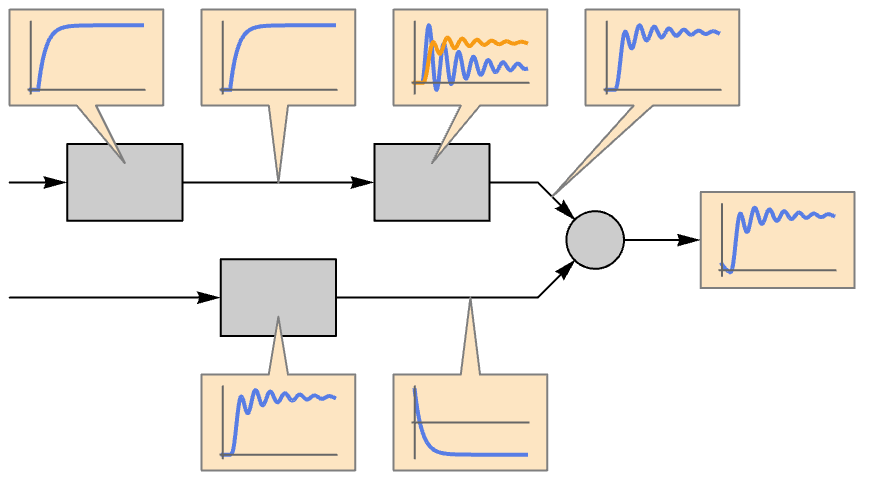
"SignalCount", "TemporalVariable"}], Table[Cos[t], {t, 0, 3π}]]Show[Plot[%, {, 0, 3π}], ListPlot[Table[{t, Cos[t]}, {t, 0, 3π}], IconizedObject[«opts»]]]InputOutputResponse[SystemsConnectionsModel[{TransferFunctionModel[{{{8}}, 8 + Control`LQDesignDump`s},
Control`LQDesignDump`s], StateSpaceModel[{{{0, 1}, {-26, -2}}, {{0}, {1}}, {{26, 0}}, {{0}}}]},
{{1, 1} -> {2, 1}}, {{1, 1}}, {{2, 1}}], 1, {t, 0, 10}]Plot[%, {t, 0, 10}, PlotRange -> All]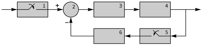
subOR = InputOutputResponse[SystemsConnectionsModel[{SamplerModel[Association["DiscreteVariables" -> {Subscript[, 1][]},
"InputVariables" -> {Subscript[, 1][]}, "OutputVariables" -> {Subscript[, 1][]},
"InitialStateValues" -> {}, "TemporalVariable" -> , "When ... Period", "SignalCount",
"TemporalVariable"}], TransferFunctionModel[{{{1}}, 1}, z, SamplingPeriod -> 0.5]},
{{1, 1} -> {2, 1}, {2, 1} -> {3, 1}, {3, 1} -> {4, 1}, {4, 1} -> {5, 1}, {5, 1} -> {6, 1},
{6, 1} -> {2, 2}}, {{1, 1}}, {{4, 1}}], Sin[t], {t, 0, 10}, "SubsystemOutputResponse"];
Short[subOR]Legended[MapIndexed[Plot[#, {t, 0, 10}, PlotStyle -> ColorData[116, #2[[1]]]]&, subOR], LineLegend[ColorData[116, "ColorList"][[1 ;; 6]], Range[6]]]特性 (11)
InputOutputResponse[SystemsConnectionsModel[{TransferFunctionModel[{{{1, -1}}, 1}, s],
  TransferFunctionModel[{{{3}}, 3 + s}, s], TransferFunctionModel[{{{7}}, 7 + s}, s]},
{{1, 1} -> {2, 1}, {2, 1} -> {3, 1}, {3, 1} -> {1, 2}}, {{1, 1}}, {{2, 1}}], 1, {t, 0, 3}, "StateResponse"]InputOutputResponse[SystemsConnectionsModel[{TransferFunctionModel[{{{1, -1}}, 1}, s],
TransferFunctionModel[{{{3}}, 3 + s}, s], TransferFunctionModel[{{{7}}, 7 + s}, s]},
{{1, 1} -> {2, 1}, {2, 1} -> {3, 1}, {3, 1} -> {1, 2}}, {{1, 1}}, {{2, 1}}], 1, {t, 0, 10}, {"StateResponse", "SubsystemOutputResponse"}]ℛ = InputOutputResponse[SystemsConnectionsModel[{TransferFunctionModel[{{{1, -1}}, 1}, s],
TransferFunctionModel[{{{3}}, 3 + s}, s], TransferFunctionModel[{{{7}}, 7 + s}, s]},
{{1, 1} -> {2, 1}, {2, 1} -> {3, 1}, {3, 1} -> {1, 2}}, {{1, 1}}, {{2, 1}}], 1, {t, 0, 10}, "Data"]ℛ["StateResponse"]ℛ["Properties"]InputOutputResponse[SystemsConnectionsModel[{TransferFunctionModel[{{{1, -1}}, 1}, s],
TransferFunctionModel[{{{3}}, 3 + s}, s], TransferFunctionModel[{{{7}}, 7 + s}, s]},
{{1, 1} -> {2, 1}, {2, 1} -> {3, 1}, {3, 1} -> {1, 2}}, {{1, 1}}, {{2, 1}}], 1, {t, 0, 10}, "PropertyAssociation"]InputOutputResponse[SystemsConnectionsModel[{TransferFunctionModel[{{{1, -1}}, 1}, s],
TransferFunctionModel[{{{3}}, 3 + s}, s], TransferFunctionModel[{{{7}}, 7 + s}, s]},
{{1, 1} -> {2, 1}, {2, 1} -> {3, 1}, {3, 1} -> {1, 2}}, {{1, 1}}, {{2, 1}}], 1, {t, 0, 10}, "PropertyDataset"]InputOutputResponse[SystemsConnectionsModel[{TransferFunctionModel[{{{1, -1}}, 1}, Control`LQDesignDump`s],
TransferFunctionModel[{{{30}}, 10 + Control`LQDesignDump`s}, Control`LQDesignDump`s],
TransferFunctionModel[{{{1, -1}}, 1}, Control`LQDesignDump`s],
Tr ... ump`s}, Control`LQDesignDump`s], TransferFunctionModel[{{{5}}, 1},
Control`LQDesignDump`s]}, {{1, 1} -> {2, 1}, {2, 1} -> {3, 1}, {3, 1} -> {4, 1},
{4, 1} -> {5, 1}, {5, 1} -> {3, 2}, {4, 1} -> {6, 1}, {6, 1} -> {1, 2}}, {{1, 1}}, {{4, 1}}], 1, {t, 0, 10}, "StateResponse"]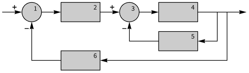
InputOutputResponse[SystemsConnectionsModel[{TransferFunctionModel[{{{1, -1}}, 1}, Control`LQDesignDump`s],
  TransferFunctionModel[{{{30}}, 10 + Control`LQDesignDump`s}, Control`LQDesignDump`s],
  TransferFunctionModel[{{{1, -1}}, 1}, Control`LQDesignDump`s],
  Tr ... ump`s}, Control`LQDesignDump`s], TransferFunctionModel[{{{5}}, 1},
   Control`LQDesignDump`s]}, {{1, 1} -> {2, 1}, {2, 1} -> {3, 1}, {3, 1} -> {4, 1},
{4, 1} -> {5, 1}, {5, 1} -> {3, 2}, {4, 1} -> {6, 1}, {6, 1} -> {1, 2}}, {{1, 1}}, {{4, 1}}], 1, {t, 0, 10}, "StateResponseAssociation"]%[4]InputOutputResponse[SystemsConnectionsModel[{TransferFunctionModel[{{{1, -1}}, 1}, Control`LQDesignDump`s],
TransferFunctionModel[{{{30}}, 10 + Control`LQDesignDump`s}, Control`LQDesignDump`s],
TransferFunctionModel[{{{1, -1}}, 1}, Control`LQDesignDump`s],
Tr ... ump`s}, Control`LQDesignDump`s], TransferFunctionModel[{{{5}}, 1},
Control`LQDesignDump`s]}, {{1, 1} -> {2, 1}, {2, 1} -> {3, 1}, {3, 1} -> {4, 1},
{4, 1} -> {5, 1}, {5, 1} -> {3, 2}, {4, 1} -> {6, 1}, {6, 1} -> {1, 2}}, {{1, 1}}, {{4, 1}}], 1, {t, 0, 10}, "OutputResponse"]InputOutputResponse[SystemsConnectionsModel[{TransferFunctionModel[{{{1, -1}}, 1}, Control`LQDesignDump`s],
TransferFunctionModel[{{{30}}, 10 + Control`LQDesignDump`s}, Control`LQDesignDump`s],
TransferFunctionModel[{{{1, -1}}, 1}, Control`LQDesignDump`s],
Tr ... ump`s}, Control`LQDesignDump`s], TransferFunctionModel[{{{5}}, 1},
Control`LQDesignDump`s]}, {{1, 1} -> {2, 1}, {2, 1} -> {3, 1}, {3, 1} -> {4, 1},
{4, 1} -> {5, 1}, {5, 1} -> {3, 2}, {4, 1} -> {6, 1}, {6, 1} -> {1, 2}}, {{1, 1}}, {{4, 1}}], 1, {t, 0, 10}, "OutputResponseAssociation"]InputOutputResponse[SystemsConnectionsModel[{TransferFunctionModel[{{{1, -1}}, 1}, Control`LQDesignDump`s],
TransferFunctionModel[{{{30}}, 10 + Control`LQDesignDump`s}, Control`LQDesignDump`s],
TransferFunctionModel[{{{1, -1}}, 1}, Control`LQDesignDump`s],
Tr ... ump`s}, Control`LQDesignDump`s], TransferFunctionModel[{{{5}}, 1},
Control`LQDesignDump`s]}, {{1, 1} -> {2, 1}, {2, 1} -> {3, 1}, {3, 1} -> {4, 1},
{4, 1} -> {5, 1}, {5, 1} -> {3, 2}, {4, 1} -> {6, 1}, {6, 1} -> {1, 2}}, {{1, 1}}, {{4, 1}}], 1, {t, 0, 10}, "SubsystemOutputResponse"]InputOutputResponse[SystemsConnectionsModel[{TransferFunctionModel[{{{1, -1}}, 1}, Control`LQDesignDump`s],
TransferFunctionModel[{{{30}}, 10 + Control`LQDesignDump`s}, Control`LQDesignDump`s],
TransferFunctionModel[{{{1, -1}}, 1}, Control`LQDesignDump`s],
Tr ... ump`s}, Control`LQDesignDump`s], TransferFunctionModel[{{{5}}, 1},
Control`LQDesignDump`s]}, {{1, 1} -> {2, 1}, {2, 1} -> {3, 1}, {3, 1} -> {4, 1},
{4, 1} -> {5, 1}, {5, 1} -> {3, 2}, {4, 1} -> {6, 1}, {6, 1} -> {1, 2}}, {{1, 1}}, {{4, 1}}], 1, {t, 0, 10}, "SubsystemOutputResponseAssociation"]%[5]特性と関係 (2)
sys = TransferFunctionModel[(3s/s^2 + 2s + 3), s]加法性には,入力の総和に対する応答は個々の入力に対する応答の和である,とある:
inps = {Sin[t], 1};InputOutputResponse[sys, Total[inps], t] - Total[Table[InputOutputResponse[sys, i, t], {i, inps}]]//Simplify均質性には,入力にスカラーをかけたものに対する応答は応答に同じスカラーをかけたものと等価である,とある:
inp = Exp[-t];InputOutputResponse[sys, c inp, t] - c InputOutputResponse[sys, inp, t]//Simplifytfm = TransferFunctionModel[{{{162}}, 2*(81 + s/2 + s^2)}, s];
Subscript[f, 1] = 1;
Short[Subscript[r, 1] = InputOutputResponse[tfm, Sin[Subscript[f, 1]t], t][[1]]]
過渡信号が消えた後で,応答は,基本的に,入力信号と同じになる:
Plot[{Sin[Subscript[f, 1]t], Subscript[r, 1]}, {t, 19, 25}, PlotRange -> All]{Subscript[m, 1], Subscript[p, 1]} = {1, 0};
Subscript[f, 2] = 20;
Short[Subscript[r, 2] = InputOutputResponse[tfm, Sin[Subscript[f, 2]t], t][[1]]]Plot[{Sin[Subscript[f, 2 ]t], Subscript[r, 2]}, {t, 19.5, 20}, PlotRange -> All]Subscript[sol, 2] = NSolve[D[Subscript[r, 2], t] == 0 && D[Subscript[r, 2], {t, 2}] < 0 && 19.5 < t < 20, t][[1]]Subscript[m, 2] = Subscript[r, 2] /. Subscript[sol, 2]Subscript[sol, i] = NSolve[D[Sin[Subscript[f, 2]t], t] == 0 && D[Sin[Subscript[f, 2]t], {t, 2}] < 0 && 19.5 < t < (t /. Subscript[sol, 2]), t][[1]]Subscript[p, 2] = (((t /. Subscript[sol, i]) - (t /. Subscript[sol, 2]))/1 / Subscript[f, 2])epM = {PointSize[Medium], Red, Point[{Log10[Subscript[f, 1]], 20 Log10[Subscript[m, 1]]}], Point[{Log10[Subscript[f, 2]], 20 Log10[Subscript[m, 2]]}]}epP = {PointSize[Medium], Red, Point[{Log10[Subscript[f, 1]], Subscript[p, 1]}], Point[{Log10[Subscript[f, 2]], Subscript[p, 2] / Degree}]}BodePlot[tfm, Epilog -> {epM, epP}, PlotLayout -> "HorizontalGrid", ImageSize -> Small]テキスト
Wolfram Research (2024), InputOutputResponse, Wolfram言語関数, https://reference.wolfram.com/language/ref/InputOutputResponse.html.
CMS
Wolfram Language. 2024. "InputOutputResponse." Wolfram Language & System Documentation Center. Wolfram Research. https://reference.wolfram.com/language/ref/InputOutputResponse.html.
APA
Wolfram Language. (2024). InputOutputResponse. Wolfram Language & System Documentation Center. Retrieved from https://reference.wolfram.com/language/ref/InputOutputResponse.html