

LQRegulatorGains
LQRegulatorGains[sspec,wts]
重みが wts の費用関数を最小化する系の指定 sspec についての状態フィードバックゲインを与える.
LQRegulatorGains[…,"prop"]
特性"prop"の値を与える.
詳細とオプション
- LQRegulatorGainsは,線形二次調整器,線形二次コントローラ,あるいは最適コントローラとしても知られている.
- LQRegulatorGainsは,調整コントローラあるいは追跡コントローラの計算に使われる.
- LQRegulatorGainsは状態入力およびフィードバック入力の二次費用関数を最小化することで作用する.
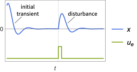
- 調整コントローラは,系を乱そうとする外乱
 があっても系を平衡状態に保とうとする.典型的な例として,直立した倒立振子や水平飛行中の航空機等が挙げられる.
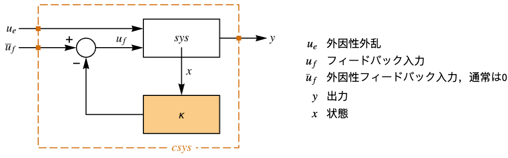
- 調整コントローラは
 の形の制御規則で与えられる.ただし,
 は計算されたゲイン行列である.
- 状態 x の重み q,r ,p およびフィードバック入力 ufの二次費用関数は以下で与えられる.
-

連続時間系 
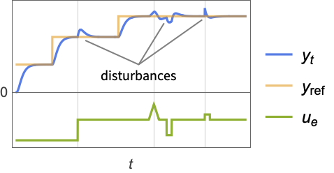
離散時間系 - 追跡コントローラは,それを妨害する外乱
 があっても参照信号を追跡しようとする.典型的な例として,自動車のクルーズコントロールシステムやロボットの経路追跡が挙げられる.
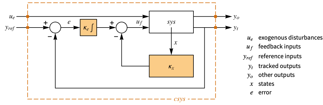
- 追跡コントローラは
 の形の制御規則で与えられる.ただし,
 は系 sys と
 のダイナミクスを含む拡張系のための計算されたゲイン行列である.
- 拡張状態
 の重み q,r ,p およびフィードバック入力 ufの二次費用関数は以下で与えられる.
-

連続時間系 
離散時間系 - 拡張系の状態の数は
 で与えられる.ただし,
 は sys のSystemsModelOrderで,
 は yrefの次数で,
 は信号 yrefの数で与えられる.
- 重み行列の選択は,結果としてパフォーマンスと制御努力のトレードオフとなり,優れた設計に反復的に到達する.初期値は成分が
 の対角行列でよい.ただし,ziは対応する xiまたは uiの許容可能な最大絶対値である.
- 重み wts は次の形でよい.
-
{q,r} クロスカップリングがない費用関数 {q,r,p} クロスカップリング行列 p がある費用関数 - LQ設計はStateSpaceModelで指定されているように線形系に使うことができる.
-

連続時間系 
離散時間系 - 結果のフィードバックゲイン行列
 は代数リッカティ(Riccati)方程式から計算される.
-

連続時間系と  は連続時間代数リッカティ方程式
 の解である

離散時間系と  は離散時間代数リッカティ方程式
 の解である
- 部分行列 bfはフィードバック入力 ufに対応する b の列である.
- 系の指定 sspec は,系 sys と指定 uf,yt,yrefである.
- 系の指定 sspec は以下の形でよい.
-
StateSpaceModel[…] 線形制御入力と線形状態 AffineStateSpaceModel[…] 線形制御入力と非線形状態 NonlinearStateSpaceModel[…] 非線形制御入力と非線形状態 SystemModel[…] 一般的な系のモデル <…> Associationとして与えられる詳細な系の指定 - 系の指定の詳細は次のキーを持つことができる.
-
"InputModel" sys モデルの任意のもの "FeedbackInputs" All フィードバック入力 uf "TrackedOutputs" None 追跡された出力 yt "TrackedSignal" Automatic yrefのダイナミクス - フィードバック入力は以下の形でよい.
-
{num1,…,numn} StateSpaceModel,AffineStateSpaceModel,NonlinearStateSpaceModelで使われる番号付きの入力 numi {name1,…,namen} SystemModelで使われる名前付きの入力 namei All すべての入力を使う - AffineStateSpaceModel,NonlinearStateSpaceModel,SystemModelのような非線形系については, 系は保存された動作点の周りで線形化される.
- LQRegulatorGains[…,"Data"]は,cd["prop"]の形で追加的な特性の抽出に使えるSystemsModelControllerDataオブジェクト cd を返す.
- LQRegulatorGains[…,"prop"]を使って cd["prop"]の値を直接得ることができる.
- 次は,特性"prop"の可能な値である.
-
"BlockDiagram" csys のブロック図 {"BlockDiagram",<"SampledData"True>} csys のサンプルデータブロック図を作成する "ClosedLoopPoles" 線形化された"ClosedLoopSystem"の極 "ClosedLoopSystem" 系 csys {"ClosedLoopSystem", cspec} 閉ループ系の形に対する詳細な制御 "ControllerModel" モデル cm "Design" コントローラ設計のタイプ "DesignModel" 設計に使われるモデル "FeedbackGains" ゲイン行列 κ またはそれに相当するもの "FeedbackGainsModel" モデル gm または{gm1,gm2} "FeedbackInputs" フィードバックに使われる sys の入力 uf "InputCount" sys の入力 u の数 "InputModel" 入力モデル sys "OpenLoopPoles" "DesignModel"の極 "OutputCount" sys の出力 y の数 "SamplingPeriod" sys のサンプリング周期 "StateCount" sys の状態 x の数 "TrackedOutputs" トラックされた sys の出力 yt - 次は,cspec の可能なキーである.
-
"InputModel" csys の入力モデル "Merge" csys をマージするかどうか "ModelName" csys の名前 "SamplingPeriod" サンプルデータ csys を作成する - 次は,調整器のレイアウトの線図である.
- 次は,追跡器のレイアウトの線図である.
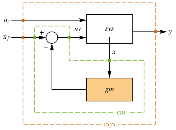
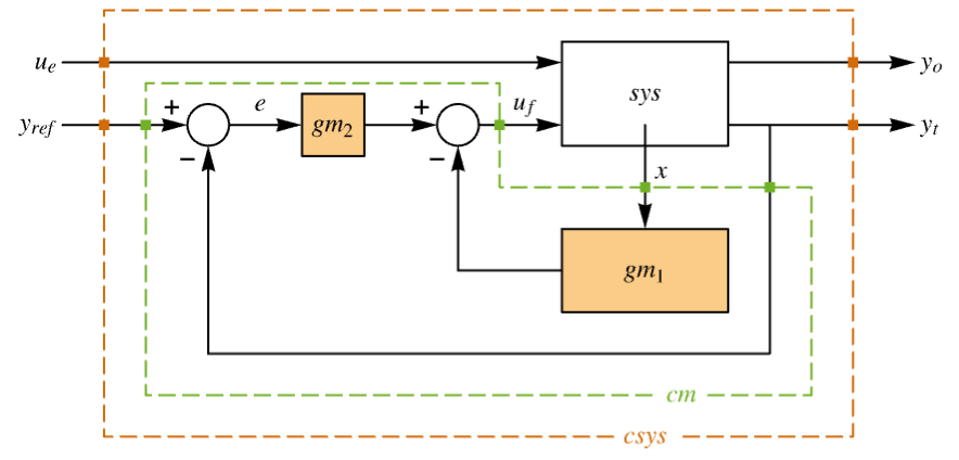
例題
すべて開く すべて閉じる例 (3)
フィードバック uf,外因性入力 ueを持つ系の指定 sspec に対する最適フィードバックゲイン:
sspec = <|"InputModel" -> StateSpaceModel[{{{2, -6}, {1., -1}}, {{6, -6}, {1, -6}}, {{0, 1}}, {{-1, 0}}},
 SamplingPeriod -> None, SystemsModelLabels ->
{{Subscript[u, f], Subscript[u, e]}}], "FeedbackInputs" -> 1|>;{q, r} = {(| | |
| - | - |
| 2 | 0 |
| 0 | 1 |), (1)};LQRegulatorGains[sspec, {q, r}]指定された制御重み wts の集合に対する非線形系のィードバックゲイン:
nssm = NonlinearStateSpaceModel[{{-1 + 2*Subscript[x, 2],
   u + 4*Subscript[x, 1] - Subscript[x, 2]},
  {Subscript[x, 1] + 3*Subscript[x, 2]}},
 {{Subscript[x, 1], 1}, {Subscript[x, 2], 1}}, {{u, 1}},
 {Automatic}, Automatic, SamplingPeriod -> None];
wts = {(|   |    |
| - | -- |
| 1 | 0  |
| 0 | 10 |), {{1}}};LQRegulatorGains[nssm, wts]//NLQRegulatorGains[StateSpaceModel[nssm], wts]//Nssm = StateSpaceModel[{{{0, 1}, {-1, 3.5}}, {{0}, {1}}, {{1, 1}}, {{0}}}, SamplingPeriod -> None,
SystemsModelLabels -> None];重み wts の指定の集合についてのコントローラデータオブジェクト:
wts = {(| | |
| --- | - |
| 100 | 0 |
| 0 | 1 |), {{1}}};𝒸𝒹 = LQRegulatorGains[ssm, wts, "Data"]PoleZeroPlot[{𝒸𝒹["InputModel"], 𝒸𝒹["ClosedLoopSystem"]}, PlotLegends -> {"o.l. poles", "o.l. zeros", "c.l. poles", "o.l. zeros"}]スコープ (34)
基本的な用法 (9)
状態と入力に等しい重みを持つ系の状態フィードバックゲインを計算する:
ssm = StateSpaceModel[{{{-10}}, {{1}}}, SamplingPeriod -> None, SystemsModelLabels -> None];
κ = LQRegulatorGains[ssm, {{{1}}, {{1}}}]SystemsModelStateFeedbackConnect[ssm, κ]//Simplifyssm = StateSpaceModel[{{{10}}, {{1}}}, SamplingPeriod -> None, SystemsModelLabels -> None];
κ = LQRegulatorGains[ssm, {{{1}}, {{1}}}]SystemsModelStateFeedbackConnect[ssm, κ]//Simplifyssm = StateSpaceModel[{{{0, 1}, {-1, -2}}, {{0}, {1}}, {{1, 0}}, {{0}}}, SamplingPeriod -> None,
SystemsModelLabels -> None];κ = LQRegulatorGains[ssm, {(| | |
| - | - |
| 1 | 0 |
| 0 | 2 |), (0.5)}]Dimensions[κ]{SystemsModelDimensions[ssm][[1]], SystemsModelOrder[ssm]}ssm = StateSpaceModel[{{{0, 0, -0.1}, {1., 0., -1.08}, {0., 1., -0.9}}, {{1, 1}, {1, 0}, {0, 0}},
{{0, 0, 1}}, {{0, 0}}}, SamplingPeriod -> None, SystemsModelLabels -> None];MatrixForm[Subscript[κ, 1] = LQRegulatorGains[ssm, {(| | | |
| - | - | -- |
| 1 | 0 | 0 |
| 0 | 1 | 0 |
| 0 | 0 | 10 |), (| | |
| - | - |
| 1 | 0 |
| 0 | 5 |)}]]MatrixForm[Subscript[κ, 2] = LQRegulatorGains[ssm, {(| | | |
| - | - | -- |
| 1 | 0 | 0 |
| 0 | 1 | 0 |
| 0 | 0 | 10 |), (| | |
| - | - |
| 5 | 0 |
| 0 | 1 |)}]]通常,より重みが大きいフィードバック入力の方がノルムが小さい:
Norm /@ Subscript[κ, 1]
Norm /@ Subscript[κ, 2]費用関数が状態入力とフィードバック入力のクロスカップリングを含む場合のゲインを計算する:
ssm = StateSpaceModel[{{{0, 0, -0.1}, {1., 0., -1.08}, {0., 1., -0.9}}, {{1, 1}, {1, 0}, {0, 0}},
{{0, 0, 1}}, {{0, 0}}}, SamplingPeriod -> None, SystemsModelLabels -> None];LQRegulatorGains[ssm, {(| | | |
| - | - | -- |
| 1 | 0 | 0 |
| 0 | 1 | 0 |
| 0 | 0 | 10 |), (| | |
| - | - |
| 1 | 0 |
| 0 | 1 |), (| | |
| ---- | --- |
| 0.1 | 0 |
| -0.2 | 0 |
| 0.15 | 0.2 |)}]//MatrixFormssm = StateSpaceModel[{{{0, 0, -0.1}, {1., 0., -1.08}, {0., 1., -0.9}}, {{1, 1}, {1, 0}, {0, 0}},
{{0, 0, 1}}, {{0, 0}}}, SamplingPeriod -> None, SystemsModelLabels -> None];wts = {(| | | |
| - | - | -- |
| 1 | 0 | 0 |
| 0 | 1 | 0 |
| 0 | 0 | 10 |), (1)};LQRegulatorGains[<|"InputModel" -> ssm, "FeedbackInputs" -> 1|>, wts]LQRegulatorGains[<|"InputModel" -> ssm, "FeedbackInputs" -> 2|>, wts]安定化可能ではあるが制御不可能である系のフィードバックゲインの集合を計算する:
LQRegulatorGains[StateSpaceModel[{{{-2, 0}, {0, 3}}, {{0}, {1}}}, SamplingPeriod -> None, SystemsModelLabels -> None], {(| | |
| - | - |
| 1 | 0 |
| 0 | 1 |), (2)}]nssm = NonlinearStateSpaceModel[{{u + x + x^2},
{-1 + x}}, {{x, 1}}, {{u, -2}}, {Automatic}, Automatic,
SamplingPeriod -> None];LQRegulatorGains[nssm, {{{10}}, {{1}}}]LQRegulatorGains[StateSpaceModel[nssm], {{{10}}, {{1}}}]費用が状態入力とフィードバック入力の二次関数として与えられた場合にゲインを計算する:
J = 2 Subsuperscript[x, 1, 2] + 2 Subsuperscript[x, 2, 2] + 5 Subsuperscript[x, 3, 2] + 0.1 Subsuperscript[u, 1, 2] + 0.2 Subsuperscript[u, 2, 2] + 2 Subscript[u, 1] Subscript[x, 1] + 2 Subscript[u, 2] Subscript[x, 2] + 10 Subscript[u, 1] Subscript[x, 3];{q, r, p} = (1/2){Subscript[∂, {{Subscript[x, 1], Subscript[x, 2], Subscript[x, 3]}, 2}]J, Subscript[∂, {{Subscript[u, 1], Subscript[u, 2]}, 2}]J, Subscript[∂, {{Subscript[x, 1], Subscript[x, 2], Subscript[x, 3]}}, {{Subscript[u, 1], Subscript[u, 2]}}]J}LQRegulatorGains[IconizedObject[«ssm»], {q, r, p}]工場モデル (6)
連続時間StateSpaceModel:
LQRegulatorGains[StateSpaceModel[{{{0, 1.}, {-1, -1.6}}, {{0}, {1}}, {{1, 1}}, {{0}}}, SamplingPeriod -> None,
SystemsModelLabels -> None], {(| | |
| - | - |
| 1 | 0 |
| 0 | 1 |), (1)}]離散時間StateSpaceModel:
LQRegulatorGains[StateSpaceModel[{{{0, 1.}, {0.020000000000000004, 0.1}}, {{0}, {1}}, {{1, 0}}, {{0}}},
SamplingPeriod -> τ, SystemsModelLabels -> None], {(| | |
| - | - |
| 1 | 0 |
| 0 | 1 |), (1)}]ディスクリプタStateSpaceModel:
LQRegulatorGains[StateSpaceModel[{{{-6, -4}, {-6, -5}}, {{1}, {1}}, {{1, 0}}, {{0}}, {{1, 1}, {0, 1}}},
{{x1[t], 0}, {x2[t], 0}},
{{u[t], 0}}, Automatic, t, SamplingPeriod -> None,
SystemsModelLabels -> None], {(| | |
| - | - |
| 1 | 0 |
| 0 | 1 |), (1.0)}]LQRegulatorGains[AffineStateSpaceModel[{{Sin[Subscript[x, 1]] + Subscript[x, 2],
-Subscript[x, 1] - Subscript[x, 2]},
{{Subscript[x, 1]}, {1}}, {Subscript[x, 1]}, {{0}}},
{Subscript[x, 1], Subscript[x, 2]}, {{u, 0}}, {Automatic},
Automatic, SamplingPeriod -> None], {(| | |
| - | - |
| 1 | 0 |
| 0 | 1 |), (1.0)}]LQRegulatorGains[NonlinearStateSpaceModel[
{{Subscript[x, 2] + Subscript[x, 1]*Subscript[x, 2],
u + Subscript[x, 1]}, {Subscript[x, 1]}},
{Subscript[x, 1], Subscript[x, 2]}, {u}, {Automatic},
Automatic, SamplingPeriod -> None], {(| | |
| - | - |
| 1 | 0 |
| 0 | 1 |), (1)}]sm = CreateSystemModel[{x''[t] + x'[t] + x[t] == u[t], y[t] == x[t]}, t, {"u"∈"Modelica.Blocks.Interfaces.RealInput", "y"∈"Modelica.Blocks.Interfaces.RealOutput"}];LQRegulatorGains[sm, {(| | |
| - | - |
| 1 | 0 |
| 0 | 1 |), (1)}]特性 (11)
LQRegulatorGainsはデフォルトでフィードバックゲインを返す:
LQRegulatorGains[StateSpaceModel[{{{0, 1}, {-1, -2}}, {{0}, {1}}, {{1, 0}}, {{0}}}, SamplingPeriod -> None,
SystemsModelLabels -> None], {(| | |
| - | - |
| 1 | 0 |
| 0 | 1 |), (1)}]% == LQRegulatorGains[StateSpaceModel[{{{0, 1}, {-1, -2}}, {{0}, {1}}, {{1, 0}}, {{0}}}, SamplingPeriod -> None,
SystemsModelLabels -> None], {(| | |
| - | - |
| 1 | 0 |
| 0 | 1 |), (1)}, "FeedbackGains"]fb = LQRegulatorGains[NonlinearStateSpaceModel[
{{-Subscript[x, 1] + u*Subscript[x, 1] +
Subscript[x, 2]/E^Subscript[x, 1],
E^Subscript[x, 2] - Subscript[x, 1]}, {Subscript[x, 2]}},
{{Subscript[x, 1], 1}, {Subscript[x, 2], 0}}, {{u, 1.}},
{Automatic}, Automatic, SamplingPeriod -> None], {(| | |
| - | - |
| 1 | 0 |
| 0 | 1 |), (1)}]κ.x+λ の形をしている.ただし,κ と λ は定数である:
{κ, λ} = {D[fb, {{Subscript[x, 1], Subscript[x, 2]}}], fb /. {Subscript[x, _] -> 0}}LQRegulatorGains[StateSpaceModel[{{{0, 1}, {-1, -2}}, {{0}, {1}}, {{1, 0}}, {{0}}}, SamplingPeriod -> None,
SystemsModelLabels -> None], {(| | |
| - | - |
| 1 | 0 |
| 0 | 1 |), (1)}, "FeedbackGainsModel"]LQRegulatorGains[NonlinearStateSpaceModel[{{Subscript[x, 2], -2/3 + u -
Subscript[x, 1]/3 - Subscript[x, 2]/2},
{Subscript[x, 1]}}, {{Subscript[x, 1], 1},
{Subscript[x, 2], 0}}, {{u, 1.}}, {Automatic}, Automatic,
SamplingPeriod -> None], {(| | |
| - | - |
| 1 | 0 |
| 0 | 1 |), (1)}, "FeedbackGainsModel"]//ChopLQRegulatorGains[StateSpaceModel[{{{0., 1.}, {-0.05, -0.9}}, {{0}, {1}}, {{1, 0}}, {{0}}},
{Subscript[x, 1], Subscript[x, 2]}, {{f, 0}},
SamplingPeriod -> None, SystemsModelLabels -> None], {(| | |
| - | - |
| 1 | 0 |
| 0 | 1 |), (1)}, "ClosedLoopSystem"]LQRegulatorGains[StateSpaceModel[{{{0., 1.}, {-0.05, -0.9}}, {{0}, {1}}, {{1, 0}}, {{0}}},
{Subscript[x, 1], Subscript[x, 2]}, {{f, 0}},
SamplingPeriod -> None, SystemsModelLabels -> None], {(| | |
| - | - |
| 1 | 0 |
| 0 | 1 |), (1)}, "BlockDiagram"]assm = AffineStateSpaceModel[{{Subscript[x, 2], -0.05*Subscript[x, 1] -
0.9*Subscript[x, 2]^2}, {{0}, {1}}, {Subscript[x, 1]}, {{0}}},
{Subscript[x, 1], Subscript[x, 2]}, {{f, 0}}, {Automatic},
Automatic, SamplingPeriod -> None];
wts = {(| | |
| - | - |
| 1 | 0 |
| 0 | 1 |), (1)};LQRegulatorGains[assm, wts, "ClosedLoopPoles"]LQRegulatorGains[assm, {(| | |
| -- | -- |
| 10 | 0 |
| 0 | 10 |), (1)}, "ClosedLoopPoles"]LQRegulatorGains[assm, {(| | |
| - | - |
| 1 | 0 |
| 0 | 1 |), (10)}, "ClosedLoopPoles"]assm = AffineStateSpaceModel[{{Subscript[x, 2], -0.05*Subscript[x, 1] -
0.9*Subscript[x, 2]^2}, {{0}, {1}}, {Subscript[x, 1]}, {{0}}},
{Subscript[x, 1], Subscript[x, 2]}, {{f, 0}}, {Automatic},
Automatic, SamplingPeriod -> None];
wts = {(| | |
| - | - |
| 1 | 0 |
| 0 | 1 |), (1)};ssm = LQRegulatorGains[assm, wts, "DesignModel"]設計モデルが入力で直接指定されているなら,フィードバックゲインの構造は異なってくる:
Table[LQRegulatorGains[m, wts], {m, {ssm, assm}}]LQRegulatorGains[AffineStateSpaceModel[{{Subscript[x, 2], -0.05*Subscript[x, 1] -
0.9*Subscript[x, 2]^2}, {{0}, {1}}, {Subscript[x, 1]}, {{0}}},
{Subscript[x, 1], Subscript[x, 2]}, {{f, 0}}, {Automatic},
Automatic, SamplingPeriod -> None], {(| | |
| - | - |
| 1 | 0 |
| 0 | 1 |), (1)}, "Design"]Dataset[Table[{prop, LQRegulatorGains[IconizedObject[«sys»], IconizedObject[«wts»], prop]}, {prop, IconizedObject[«props»]}]]𝒸𝒹 = LQRegulatorGains[IconizedObject[«sys»], IconizedObject[«wts»], "Data"]𝒸𝒹["Properties"]𝒸𝒹["ClosedLoopPoles"]追跡 (5)
sspec = <|"InputModel" -> StateSpaceModel[{{{0, 1}, {-5, -3}}, {{0}, {1}}, {{5, 0}}, {{0}}}, SamplingPeriod -> None,
SystemsModelLabels -> None], "TrackedOutputs" -> 1|>;𝒸𝒹 = LQRegulatorGains[sspec, {(| | | |
| - | - | --- |
| 1 | 0 | 0 |
| 0 | 1 | 0 |
| 0 | 0 | 100 |), {{0.1}}}, "Data"]
OutputResponse[𝒸𝒹["ClosedLoopSystem"], 1, {t, 0, 3}];
Plot[{1, %}, {t, 0, 3}, IconizedObject[«plotOpts»]]sspec = <|"InputModel" -> StateSpaceModel[{{{0, 1.}, {0.5, -2.3}}, {{0}, {1.}}, {{1., 0}}, {{0}}}, SamplingPeriod -> 0.1,
SystemsModelLabels -> None], "TrackedOutputs" -> 1|>;𝒸𝒹 = LQRegulatorGains[sspec, {(| | | |
| - | - | - |
| 1 | 0 | 0 |
| 0 | 1 | 0 |
| 0 | 0 | 1 |), {{0.1}}}, "Data"]
ref = Table[1, 15];
OutputResponse[𝒸𝒹["ClosedLoopSystem"], ref];
ListLinePlot[{ref, %[[1]]}, IconizedObject[«plotOpts»]]𝒸𝒹["BlockDiagram"]sspec = <|"InputModel" -> StateSpaceModel[{{{2., 0}, {0, -2}}, {{1., 0}, {0, 1}}, {{1, 0}, {3., 1}}, {{0, 0}, {0, 0}}},
SamplingPeriod -> None, SystemsModelLabels -> None], "TrackedOutputs" -> {1, 2}|>;𝒸𝒹 = LQRegulatorGains[sspec, N@{(| | | | |
| - | - | -- | -- |
| 1 | 0 | 0 | 0 |
| 0 | 1 | 0 | 0 |
| 0 | 0 | 50 | 0 |
| 0 | 0 | 0 | 30 |), (| | |
| - | - |
| 1 | 0 |
| 0 | 1 |)}, "Data"]refs = RandomInteger[{-7, -1}, 2];
or = OutputResponse[𝒸𝒹["ClosedLoopSystem"], refs, {t, 0, 10}];Plot[Evaluate[Riffle[refs, or]], {t, 0, 10}, IconizedObject[«plotOpts»]]sspec = <|"InputModel" -> StateSpaceModel[{{{0, 1}, {-5, -3}}, {{0}, {1}}, {{5, 0}}, {{0}}}, SamplingPeriod -> None,
SystemsModelLabels -> None], "TrackedOutputs" -> 1|>;𝒸𝒹 = LQRegulatorGains[sspec, {(| | | |
| -- | - | -- |
| 10 | 0 | 0 |
| 0 | 1 | 0 |
| 0 | 0 | 10 |), {{0.1}}}, "Data"]cm = 𝒸𝒹["ControllerModel"]ref = {1};
csys = 𝒸𝒹["ClosedLoopSystem"];
n = SystemsModelOrder[sspec["InputModel"]];cinps = Join[ref, OutputResponse[csys, ref, {t, 0, 5}], StateResponse[csys, ref, {t, 0, 5}][[1 ;; n]]]OutputResponse[cm, cinps, {t, 0, 5}];
Plot[%, {t, 0, 5}, PlotRange -> All]tSig = Function[{r, t}, r''[t] + r[t]]m = Max[Join[Cases[tSig[r, t], Derivative[n_][r][t] :> n], {0}]]ref = r[t] /. DSolve[Join[{tSig[r, t] == 0}, {r[0] == 1, r'[0] == 0}], r[t], t]sspec = <|"InputModel" -> StateSpaceModel[{{{-1}}, {{1}}, {{1}}, {{0}}}, SamplingPeriod -> None, SystemsModelLabels -> None], "TrackedOutputs" -> {1}, "TrackedSignal" -> tSig|>;{q, k} = {Length[sspec["TrackedOutputs"]], SystemsModelOrder[sspec["InputModel"]]}{qq, rr} = {(| | | |
| - | - | - |
| 1 | 0 | 0 |
| 0 | 1 | 0 |
| 0 | 0 | 1 |), {{0.1}}};
Join[Dimensions[qq], {k + m q}]𝒸𝒹 = LQRegulatorGains[sspec, {qq, rr}, "Data"]OutputResponse[𝒸𝒹["ClosedLoopSystem"], ref, {t, 0, 10}];
Plot[{ref, %}, {t, 0, 10}, IconizedObject[«plotOpts»]]閉ループ系 (3)
assm = AffineStateSpaceModel[{{Subscript[x, 1] + Subscript[x, 2],
   -Subscript[x, 1]^3 - Subscript[x, 2]}, {{0}, {1}},
  {Subscript[x, 1]}, {{0}}}, {Subscript[x, 1],
Subscript[x, 2]}, {u}, {Automatic}, Automatic, SamplingPeriod -> None];Subscript[csys, 1] = LQRegulatorGains[assm, {(| | |
| - | - |
| 1 | 0 |
| 0 | 1 |), (1.0)}, "ClosedLoopSystem"]Subscript[csys, 2] = LQRegulatorGains[StateSpaceModel[assm], {(| | |
| - | - |
| 1 | 0 |
| 0 | 1 |), (1.0)}, "ClosedLoopSystem"]Table[OutputResponse[{sys, {0.5, 1}}, 0, {t, 0, 7}], {sys, {Subscript[csys, 1], Subscript[csys, 2]}}];
Plot[%, {t, 0, 7}, IconizedObject[«plotOpts»]]1つの外乱と1つのフィードバック入力を持つ工場のマージされた閉ループを組み立てる:
sys = <|"InputModel" -> StateSpaceModel[{{{0., 1.}, {-0.05, -0.9}}, {{0, 0}, {1, 1}}, {{1, 0}}, {{0, 0}}},
 {Subscript[x, 1], Subscript[x, 2]},
 {{d, 0}, {f, 0}}, SamplingPeriod -> None,
 SystemsModelLabels -> {{Subscript[u, e],
Subscript[u, f]}}], "FeedbackInputs" -> 2|>;wts = {(| | |
| - | - |
| 1 | 0 |
| 0 | 1 |), (1.0)};LQRegulatorGains[sys, wts, "ClosedLoopSystem"]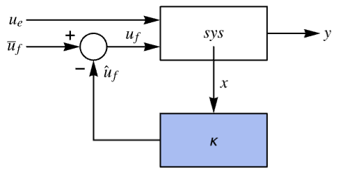
LQRegulatorGains[sys, wts, {"ClosedLoopSystem", <|"Merge" -> False|>}]SystemsModelMerge[%]LQRegulatorGains[sys, wts, {"ClosedLoopSystem", <|"Merge" -> True|>}]sm = CreateSystemModel["RLC", {ℒ q''[t] + ℛ q'[t] + q[t] / 𝒞 == e[t], y[t] == q'[t]}, t, {"e"∈"Modelica.Blocks.Interfaces.RealInput", "y"∈"Modelica.Blocks.Interfaces.RealOutput"}, <|"ParameterValues" -> {ℒ -> 1, ℛ -> 1, 𝒞 -> 1}|>];csysName = "RLCWithStateFeedback";csys = LQRegulatorGains[sm, IconizedObject[«wts»], {"ClosedLoopSystem", <|"ModelName" -> csysName|>}]csys["ModelName"]この名前を直接使って他の関数で閉ループモデルを指定することができる:
SystemModelSimulate[csysName, {"y"}, 10, <|"Inputs" -> {"e" -> (5UnitStep[#]&)}|>]SystemModelPlot[%, All, PlotRange -> All]アプリケーション (11)
力学系 (2)
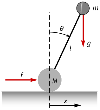
segw = NonlinearStateSpaceModel[IconizedObject[«eqns»] /. IconizedObject[«pars»], {x[t], x'[t], θ[t], θ'[t]}, f[t], {x[t], θ[t]}, t]//FullSimplifyOutputResponse[{segw, {0, 0, 3.13}}, 0, {t, 0, 20}];
GraphicsRow[Table[Plot[or[[1]], {t, 0, 0.8}, IconizedObject[«plotOpts»]], {or, ({%, {"x", "θ"}})}]]segw = NonlinearStateSpaceModel[segw, Automatic, Automatic, Automatic, None];dssm = ToDiscreteTimeModel[segw, τ = 0.05]//Simplifywts = {DiagonalMatrix[{500, 10, 20, 10}], {{0.05}}};𝒸𝒹 = LQRegulatorGains[dssm, wts, "Data"]dcsys = 𝒸𝒹["ClosedLoopSystem"]//Simplifyn = 200;sr = StateResponse[{dcsys, {0, 0, 3, 0}}, Table[0, n]];
ListStepPlot[%[[1]], DataRange -> {0, (n - 1) τ}, PlotRange -> All]cm = 𝒸𝒹["ControllerModel"]OutputResponse[cm, Join[Table[{0}, n], sr]];
ListStepPlot[%, DataRange -> {0, (n - 1)τ}, PlotRange -> All]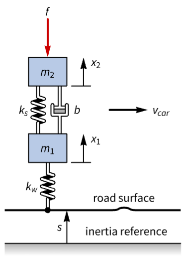
susp = StateSpaceModel[IconizedObject[«eqns»] /. IconizedObject[«pars»], {Subscript[x, 1][t], Subscript[x, 2][t]}, {s[t], f[t]}, Subscript[x, 2][t], t, IconizedObject[«labels»]]OutputResponse[susp, {0.1 UnitBox[t - 1], 0}, {t, 0, 7}];
Plot[%, {t, 0, 7}, PlotRange -> All]アクティブな減衰力を唯一のフィードバック入力として設定する:
sspec = <|"InputModel" -> susp, "FeedbackInputs" -> 2|>;wts = {DiagonalMatrix[{1, 1, 10^11, 1}], {{50.}}};𝒸𝒹 = LQRegulatorGains[sspec, wts, "Data"]csys = 𝒸𝒹["ClosedLoopSystem"]sr = StateResponse[{csys, {0, 13, 0, 8}}, {0, 0}, {t, 0, 2}];
Plot[%[[3]], {t, 0, 2}, PlotRange -> All]OutputResponse[𝒸𝒹["ControllerModel"], Join[{0}, sr], {t, 0, 2}];
Plot[%, {t, 0, 2}, PlotRange -> All]電気機械系 (4)
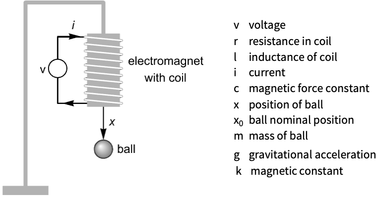

assm = AffineStateSpaceModel[IconizedObject[«eqns»], {{x[t], Subscript[x, 0]}, {x'[t], 0},
{i[t], Subscript[x, 0] Sqrt[(m g/k)]}}, {{v[t], r Subscript[x, 0] Sqrt[(m g/k)]}}, x[t], t] /. IconizedObject[«pars»]OutputResponse[{assm, {RandomInteger[{1, 10}], 0, 0}}, 0, {t, 0, 5}];
Plot[%, {t, 0, 5}]sspec = <|"InputModel" -> AffineStateSpaceModel[assm, Automatic, Automatic, Automatic, None], "FeedbackInputs" -> 1|>;ボールを浮揚させるためのフィードバックコントローラを設計する:
𝒸𝒹 = LQRegulatorGains[sspec, {(|     |     |     |
| --- | --- | --- |
| 0.1 | 0   | 0   |
| 0   | 0.1 | 0   |
| 0 | 0 | 0.1 |), {{5}}}, "Data"]csys = 𝒸𝒹["ClosedLoopSystem"]//Simplify
sr = StateResponse[{csys, {0.8, 0, 0}}, 0, {t, 0, 2}];
Plot[{%[[1]], 0.5}, {t, 0, 2}, IconizedObject[«plotOpts»]]Table[Plot[j[[1]], {t, 0, 2}, IconizedObject[«plotOpts»]], {j, Thread[{sr[[2 ;; 3]], {x', i}}]}]cm = 𝒸𝒹["ControllerModel"]OutputResponse[cm, Join[{0}, sr], {t, 0, 2}];
Plot[%, {t, 0, 2}, PlotRange -> All]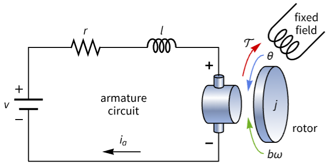
motor = StateSpaceModel[IconizedObject[«eqns»] /. IconizedObject[«pars»], {θ[t], ω[t], Subscript[i, a][t]}, {v[t], 𝒯[t]}, θ[t], t, IconizedObject[«labels»]]OutputResponse[motor, {0, 0.1DiracDelta[t - 1]}, {t, 0, 5}];
Plot[%, {t, 0, 5}, PlotRange -> All]sspec = <|"InputModel" -> motor, "FeedbackInputs" -> 1|>;
𝒸𝒹 = LQRegulatorGains[sspec, {(| | | |
| --- | - | - |
| 100 | 0 | 0 |
| 0 | 5 | 0 |
| 0 | 0 | 1 |), {{0.01}}}, "Data"]csys = 𝒸𝒹["ClosedLoopSystem"]sr = StateResponse[{csys, {0, 0.25}}, {0, 0}, {t, 0, 10}];
Plot[sr[[1]], {t, 0, 10}, PlotRange -> All]OutputResponse[𝒸𝒹["ControllerModel"], Join[{0}, sr], {t, 0, 10}];
Plot[%, {t, 0, 10}, PlotRange -> All]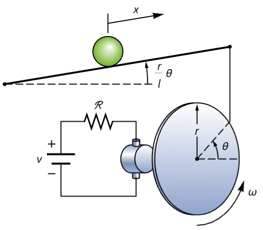
bbs = NonlinearStateSpaceModel[IconizedObject[«eqns»] /. IconizedObject[«pars»], {x[t], x'[t], θ[t], ω[t]}, v[t], {x[t], θ[t]}, t]//SimplifydBbs = ToDiscreteTimeModel[bbs, τ = 0.1]//SimplifyOutputResponse[{dBbs, {0.1, 0, 0.5, 0}}, Table[0, 20]];
ListStepPlot[%, DataRange -> {0, 19 τ}, IconizedObject[«plotOpts»]]ボールをもとの位置に戻す状態フィードバックコントローラを設計する:
dBbs = NonlinearStateSpaceModel[dBbs, Automatic, Automatic, Automatic, None];𝒸𝒹 = LQRegulatorGains[dBbs, {(| | | | |
| ---- | --- | ---- | --- |
| 10^7 | 0 | 0 | 0 |
| 0 | 500 | 0 | 0 |
| 0 | 0 | 10^5 | 0 |
| 0 | 0 | 0 | 500 |), {{10^3}}}, "Data"]csys = Simplify[𝒸𝒹["ClosedLoopSystem"]]sr = StateResponse[{csys, {0.1, 0, 0.25, 0}}, Table[0, 90]];
Table[ListStepPlot[𝓈𝓇[[1]], DataRange -> {0, 89 τ}, IconizedObject[«plotOpts»]], {𝓈𝓇, ({sr, {x, x', θ, ω}})}]OutputResponse[𝒸𝒹["ControllerModel"], Join[{Table[0, 90]}, sr]];
ListStepPlot[%, DataRange -> {0, 89 τ}, PlotRange -> All]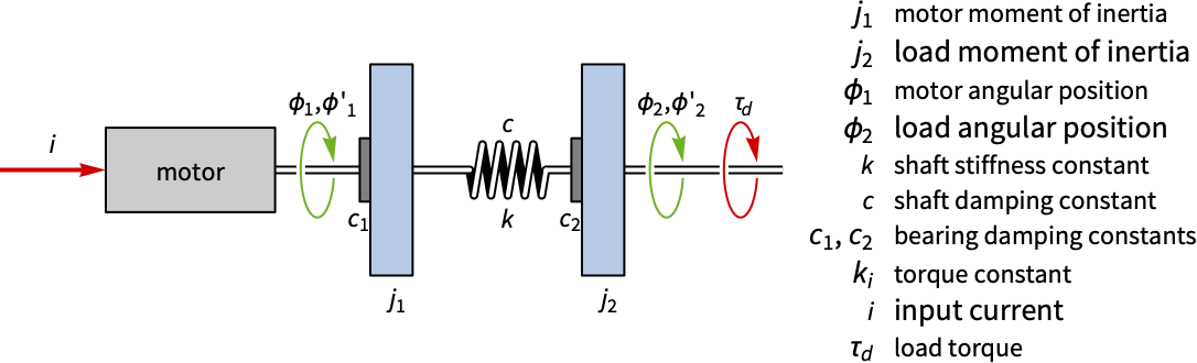
shaft = StateSpaceModel[IconizedObject[«eqns»] /. IconizedObject[«pars»], {Subscript[ϕ, 1][t], Subscript[ϕ, 2][t], Derivative[1][Subscript[ϕ, 1]][t], Derivative[1][Subscript[ϕ, 2]][t]}, {i[t], Subscript[τ, d][t]}, {Derivative[1][Subscript[ϕ, 1]][t], Derivative[1][Subscript[ϕ, 2]][t]}, t, IconizedObject[«labels»]]tSig = Function[{r, t}, r''[t] + r[t]];
ref = r[t] /. DSolve[Join[{tSig[r, t] == 0}, {r[0] == 0, r'[0] == 1}], r[t], t][[1]]電流を唯一の入力として,正弦波信号を追跡信号として設定する:
sspec = <|"InputModel" -> shaft, "FeedbackInputs" -> 1, "TrackedOutputs" -> 1, "TrackedSignal" -> tSig|>;wts = {DiagonalMatrix[{10, 1, 1, 10^3, 1, 10^2}], {{0.1}}};𝒸𝒹 = LQRegulatorGains[sspec, wts, "Data"]csys = 𝒸𝒹["ClosedLoopSystem"]sr = StateResponse[csys, {0, ref}, {t, 0, 60}];
Plot[{ref, %[[3]]}, {t, 0, 30}, IconizedObject[«plotOpts»]]cm = 𝒸𝒹["ControllerModel"]//ChopShort[cinps = Join[{ref, sr[[3]]}, sr]]OutputResponse[cm, cinps, {t, 0, 60}];
Plot[%, {t, 0, 30}, PlotRange -> All]航空宇宙系 (2)
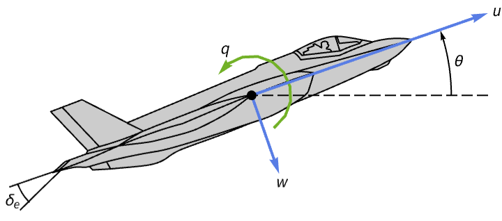
aircraft = StateSpaceModel[IconizedObject[«eqns»] /. IconizedObject[«pars»], {u[t], w[t], q[t], θ[t]}, Subscript[δ, e][t],
	θ[t], t, IconizedObject[«labels»]]
ピッチ角の外乱に対する開ループ応答は安定するまでにおよそ 秒かかる:
OutputResponse[{aircraft, {0, 0, 0, -0.1}}, 0, {t, 0, 2000}];
Plot[%, {t, 0, 2000}, PlotRange -> All]𝒸𝒹 = LQRegulatorGains[aircraft, {DiagonalMatrix[{0, 0, 0, 2.5}], {{1}}}]ℓ = EstimatorGains[aircraft, {-2 + 3I, -2 - 3I, -1, -0.05}]ℯ𝓇 = EstimatorRegulator[aircraft, {ℓ, 𝒸𝒹}, "Data"]csys = ℯ𝓇["ClosedLoopSystem"]or = OutputResponse[{csys, {0, 0, 0, -0.1}}, 0, {t, 0, 20}];
Plot[or, {t, 0, 20}, PlotRange -> All]OutputResponse[ℯ𝓇["ControllerModel"], Join[{0}, or], {t, 0, 20}];
Plot[%, {t, 0, 20}, PlotRange -> All]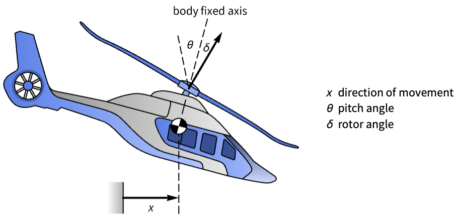
helicopter = StateSpaceModel[IconizedObject[«eqns»] /. IconizedObject[«pars»], {x[t], θ[t]}, δ[t], θ[t], t, IconizedObject[«labels»]]
TransferFunctionPoles[TransferFunctionModel[helicopter]][[1, 1]];
Count[%, _ ? (Re[#] >= 0&)]StateResponse[{helicopter, {0, 0, 0.02}}, 0, {t, 0, 2}];
Table[Plot[𝓈𝓇[[1]], {t, 0, 2}, IconizedObject[«plotOpts»]], {𝓈𝓇, ({%, {x, x', θ, θ'}})}]𝒸𝒹 = LQRegulatorGains[helicopter, {(| | | | |
| ---- | -- | ---- | - |
| 10^4 | 0 | 0 | 0 |
| 0 | 10 | 0 | 0 |
| 0 | 0 | 10^4 | 0 |
| 0 | 0 | 0 | 1 |), {{10^3}}}, "Data"]csys = 𝒸𝒹["ClosedLoopSystem"]Count[𝒸𝒹["ClosedLoopPoles"], _ ? (Re[#] >= 0&)]sr = StateResponse[{csys, {0, 0, 0.02}}, 0, {t, 0, 10}];
Table[Plot[𝓈𝓇[[1]], {t, 0, 10}, IconizedObject[«plotOpts»]], {𝓈𝓇, ({%, {x, x', θ, θ'}})}]OutputResponse[𝒸𝒹["ControllerModel"], Join[{0}, sr], {t, 0, 10}];
Plot[%, {t, 0, 10}, PlotRange -> All]電気系 (1)
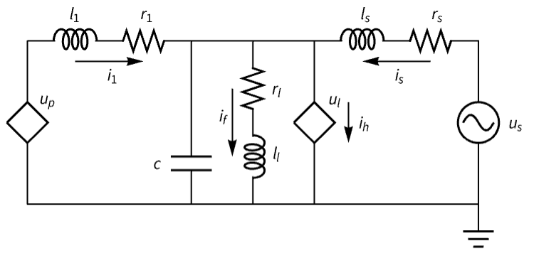
apf = StateSpaceModel[IconizedObject[«abc»], IconizedObject[«labels»]] /. IconizedObject[«pars»]PoleZeroPlot[apf]しかし,系の応答は1000rad/sに近い周波数でほぼ共振している:
BodePlot[apf, PlotLayout -> "Magnitude"]応答を調整するためにゲインを上げてコントローラーの集合を設計する:
sspec = <|"InputModel" -> apf, "FeedbackInputs" -> 1|>;𝒸𝒹 = Table[LQRegulatorGains[sspec, {DiagonalMatrix[{q, 1, 1, 1}], {{1}}}, "Data"], {q, {10, 10^3, 10^6}}]csys = Table[𝒸𝒹[[i]]["ClosedLoopSystem"], {i, 3}]Grid[Through[𝒸𝒹["ClosedLoopPoles"]], Frame -> True]PoleZeroPlot[csys, AspectRatio -> 1]重みが増加するにつれて,応答は1000rad/s近くでより減衰するようになた:
Grid[{Table[BodePlot[i[[1]], ...], {i, Thread[{csys, {q = 10, q = 10^3, q = 10^6}}]}]}]化学系 (1)
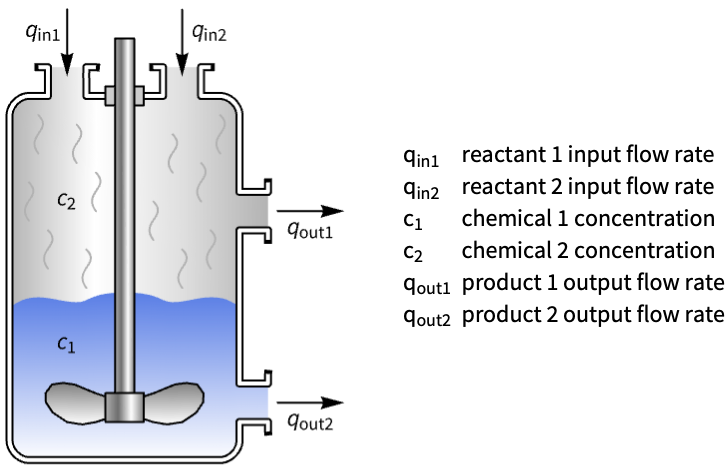
τ = 5;
tank = StateSpaceModel[IconizedObject[«abc»], SamplingPeriod -> τ, IconizedObject[«labels»]]OutputResponse[{tank, {0.1, -0.001}}, Table[{0, 0}, 100]];
ListStepPlot[%, DataRange -> {0, 99 τ}, IconizedObject[«plotOpts»]]𝒸𝒹 = LQRegulatorGains[tank, {(| | |
| - | ---- |
| 1 | 0 |
| 0 | 10^3 |), (| | |
| - | - |
| 1 | 0 |
| 0 | 1 |)}, "Data"]csys = 𝒸𝒹["ClosedLoopSystem"]sr = StateResponse[{csys, {0.1, -0.001}}, Table[{0, 0}, 10]];
Table[ListStepPlot[𝓈𝓇[[1]], DataRange -> {0, 9 τ}, IconizedObject[«plotOpts»]], {𝓈𝓇, ({%, {Subscript[c, 1], Subscript[c, 2]}})}]OutputResponse[𝒸𝒹["ControllerModel"], Join[Table[{0, 0}, 10], sr]];
Table[ListStepPlot[ℴ𝓇[[1]], DataRange -> {0, 9 τ}, IconizedObject[«plotOpts»]], {ℴ𝓇, ({%, {Subscript[q, out1], Subscript[q, out2]}})}]航海 (1)
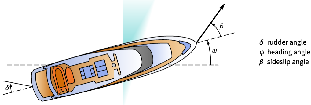
boat = StateSpaceModel[IconizedObject[«abc»], IconizedObject[«labels»]]TransferFunctionPoles[TransferFunctionModel[boat]][[1, 1]]OutputResponse[{boat, {0, 0.01, 0.2}}, 0, {t, 0, 240}];
Plot[%, {t, 0, 240}, PlotRange -> All]𝒸𝒹 = LQRegulatorGains[boat, {5000(| | | |
| - | - | - |
| 1 | 0 | 0 |
| 0 | 1 | 0 |
| 0 | 0 | 5 |), {{2500}}}, "Data"]csys = 𝒸𝒹["ClosedLoopSystem"]sr = StateResponse[{csys, {0, 0.01, 0.2}}, 0, {t, 0, 60}];
Plot[%[[3]], {t, 0, 60}, PlotRange -> All]cm = 𝒸𝒹["ControllerModel"]OutputResponse[cm, Join[{0}, sr], {t, 0, 60}];
Plot[%, {t, 0, 60}, PlotRange -> All]特性と関係 (24)
状態フィードバックゲインは負のフィードバックについて計算される:
a = RandomReal[{-1, 1}, {2, 2}];
b = RandomReal[{-1, 1}, {2, 1}];
wts = {DiagonalMatrix[RandomReal[{1, 10}, 2]], RandomReal[{1, 10}, {1, 1}]};𝒸𝒹 = LQRegulatorGains[StateSpaceModel[{a, b}], wts, "Data"]
κ  = 𝒸𝒹["FeedbackGains"];
p = Eigenvalues[a - b.κ]ContainsExactly[p, 𝒸𝒹["ClosedLoopPoles"], SameTest -> (Chop[#1 - #2] == 0. &)]𝒸𝒹 = LQRegulatorGains[StateSpaceModel[{{{-1, 2}, {1, 3}}, {{1}, {0}}}, SamplingPeriod -> None, SystemsModelLabels -> None], {(| | |
| - | --- |
| 1 | 0 |
| 0 | 0.1 |), (0.5)}, "Data"]SystemsModelStateFeedbackConnect[𝒸𝒹["InputModel"], 𝒸𝒹["FeedbackGains"]]𝒸𝒹["ClosedLoopSystem"]
nsys = NonlinearStateSpaceModel[{{-2*Subscript[x, 1] + Subscript[x, 1]^2 +
Subscript[x, 2], 1 + u - Subscript[x, 1] -
Subscript[x, 2] + Subscript[x, 1]*Subscript[x, 2]},
{Subscript[x, 1]}}, {{Subscript[x, 1], 1},
{Subscript[x, 2], 1}}, {u}, {Automatic}, Automatic,
SamplingPeriod -> None];
wts = {(| | |
| -- | -- |
| .1 | 0 |
| 0 | 10 |), (1)};LQRegulatorGains[nsys, wts]
κ = LQRegulatorGains[StateSpaceModel[nsys], wts]//N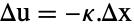
-SolveValues[{u - 0} == -κ.{Subscript[x, 1] - 1, Subscript[x, 2] - 1}, u]//Simplifyssm = StateSpaceModel[{{{0, 1}, {-16, -5.6}}, {{0}, {16}}}, SamplingPeriod -> None,
SystemsModelLabels -> None];
wts = {(| | |
| -- | -- |
| 10 | 0 |
| 0 | 10 |), (1)};fgm = LQRegulatorGains[ssm, wts, "FeedbackGainsModel"]lgm = SystemsModelSeriesConnect[ssm, fgm]
Last /@ GainMargins[lgm]
Last /@ PhaseMargins[lgm] / Degreeこれは,ナイキスト線図が常に を中心とする単位円の外側にあるからである:
lgms = Table[SystemsModelSeriesConnect[ssm, LQRegulatorGains[ssm, {DiagonalMatrix[RandomReal[{100, 1000}, 2]], RandomReal[{10, 100}, {1, 1}]}, "FeedbackGainsModel"]], 3];Show[Graphics[{LightGray, Disk[{-1, 0}]}], NyquistPlot[lgms], Axes -> True]制御可能な標準StateSpaceModelは状態フィードバックを使って完全に制御できる:
ssm = StateSpaceModel[{{{0, 1}, {-1, -2}}, {{0}, {1}}}, SamplingPeriod -> None,
SystemsModelLabels -> None];ControllableModelQ[ssm]cd = LQRegulatorGains[ssm, {(| | |
| -- | -- |
| 10 | 0 |
| 0 | .1 |), (2)}, "Data"];
cd["FeedbackGains"]cd[{"ClosedLoopPoles", "OpenLoopPoles"}]制御可能な非特異記述子StateSpaceModelも完全に制御できる:
dssm = StateSpaceModel[{{{1, 1}, {0, 0}}, {{0}, {1}}, {{1, 0}}, {{0}}, {{1, 0}, {1, 1}}},
SamplingPeriod -> None, SystemsModelLabels -> None];{ControllableModelQ[dssm], MatrixRank[Last[Normal[dssm]]]}cd = LQRegulatorGains[dssm, {(| | |
| -- | -- |
| 10 | 0 |
| 0 | .1 |), {{2}}}, "Data"];
cd["FeedbackGains"]cd[{"ClosedLoopPoles", "OpenLoopPoles"}]制御不可能な標準StateSpaceModelの部分系のみが制御可能である:
ssm = StateSpaceModel[{{{-2., 0}, {0, -1}}, {{1}, {0}}, {{1, 1}}, {{0}}}, SamplingPeriod -> None,
 SystemsModelLabels -> None];

modes = Eigenvalues[First[Normal[ssm]]];
Table[{λ, ControllableModelQ[{ssm, {λ}}]}, {λ, modes}]
LQRegulatorGains[ssm, {RandomReal[{10, 100}](|   |   |
| - | - |
| 1 | 0 |
| 0 | 1 |), {{1}}}, {"OpenLoopPoles", "ClosedLoopPoles"}]dssm = StateSpaceModel[{{{-5, 0}, {0, 1}}, {{1}, {0}}, {{1, 0}}, {{0}}, {{1, 0}, {0, 0}}},
SamplingPeriod -> None, SystemsModelLabels -> None];
ControllableModelQ[{dssm, "Slow"}]dim = Total[Diagonal[Normal[dssm][[5]]]]wts = {RandomReal[{10, 100}](| | |
| - | - |
| 1 | 0 |
| 0 | 1 |), {{1}}}
𝒸𝒹 = LQRegulatorGains[dssm, wts, "Data"];
𝒸𝒹["FeedbackGains"]
遅い部分系の極は移動されるが,速い部分系の にある極は変化しない:
{𝒸𝒹["OpenLoopPoles"], 𝒸𝒹["ClosedLoopPoles"]}{ControllableModelQ[dssm], SystemsModelOrder[dssm]}制御不可能な遅い部分系を持つ非特異記述子系は全く制御できない:
dssm = StateSpaceModel[{{{-5, 0}, {0, 1}}, {{0}, {0}}, {{1, 0}}, {{0}}, {{1, 0}, {0, 0}}},
 SamplingPeriod -> None, SystemsModelLabels -> None];
ControllableModelQ[{dssm, "Slow"}]dim = Total[Diagonal[Normal[dssm][[5]]]]p = {RandomReal[{10, 100}](| | |
| - | - |
| 1 | 0 |
| 0 | 1 |), {{1}}}LQRegulatorGains[dssm, p, {"OpenLoopPoles", "ClosedLoopPoles"}]ssm = StateSpaceTransform[StateSpaceModel[{{{1, 0}, {0, -4}}, {{1}, {0}}}], RandomReal[{-1, 1}, {2, 2}]]eigs = Eigenvalues[First[Normal[ssm]]]unstableEig = Cases[eigs, _ ? NonNegative]{ControllableModelQ[ssm], ControllableModelQ[{ssm, unstableEig}]}LQRegulatorGainsは系の安定化ゲインが計算できる:
wts = {RandomReal[{1, 10}](|   |   |
| - | - |
| 1 | 0 |
| 0 | 1 |), {{RandomReal[]}}};
cd = LQRegulatorGains[ssm, wts, "Data"];cd["FeedbackGains"]状態フィードバックは不安定な固有値を左半平面にもたらし,他の半空間を変更せずに残す:
cd["ClosedLoopPoles"]連続時間系については,ゲインはRiccatiSolveを使って計算される:
{a, b} = {(| | |
| - | --- |
| 0 | 1 |
| 0 | -10 |), (| |
| - |
| 0 |
| 1 |)};
{q, r, p} = {(| | |
| --- | - |
| 100 | 0 |
| 0 | 1 |), (1), (| |
| --- |
| 0.5 |
| 1 |)};r^-1.(b.RiccatiSolve[{a, b}, {q, r, p}] + p)LQRegulatorGainsも同じ結果を与える:
LQRegulatorGains[StateSpaceModel[{a, b}], {q, r, p}]離散時間系については,ゲインはDiscreteRiccatiSolveを使って計算される:
{a, b} = {(| | |
| - | ---- |
| 0 | 0.2 |
| 0 | -0.1 |), (| |
| --- |
| 0 |
| 0.5 |)};
{q, r, p} = {(| | |
| --- | - |
| 100 | 0 |
| 0 | 1 |), (1), (| |
| --- |
| 0.5 |
| 1 |)};With[{x = DiscreteRiccatiSolve[{a, b}, {q, r, p}]}, (b.x.b + r)^-1.(b.x.a + p)]LQRegulatorGainsも同じ結果を与える:
LQRegulatorGains[StateSpaceModel[{a, b}, SamplingPeriod -> τ], {q, r, p}]𝒸𝒹 = Table[LQRegulatorGains[StateSpaceModel[{{{0.5}}, {{1}}}, SamplingPeriod -> None, SystemsModelLabels -> None], {(w), (1)}, "Data"], {w, {10, 1}}];sr = Table[StateResponse[{𝒸𝒹[[i]]["ClosedLoopSystem"], 0.1}, 0, {t, 0, 5}], {i, 2}];
Plot[sr, {t, 0, 5}, PlotRange -> All, PlotLegends -> {"q=10", "q=1"}]Table[-𝒸𝒹[[i]]["FeedbackGains"].sr[[i]], {i, 2}];
Plot[%, {t, 0, 5}, PlotRange -> All, PlotLegends -> {"q=10", "q=1"}]𝒸𝒹 = Table[LQRegulatorGains[StateSpaceModel[{{{0.5}}, {{1}}}, SamplingPeriod -> None, SystemsModelLabels -> None], {(1), (w)}, "Data"], {w, {10, 1}}];sr = Table[StateResponse[{𝒸𝒹[[i]]["ClosedLoopSystem"], 0.1}, 0, {t, 0, 8}], {i, 2}];
Plot[sr, {t, 0, 8}, PlotLegends -> {"q=10", "q=1"}]Table[-𝒸𝒹[[i]]["FeedbackGains"].sr[[i]], {i, 2}];
Plot[%, {t, 0, 8}, PlotRange -> All, PlotLegends -> {"q=10", "q=1"}]安定した系では,制御重みが大きくなると閉ループ極が開ループ極に近付く:
wts = {0.1, 1, 10, 1000, 10000};Subscript[p, cl] = Table[LQRegulatorGains[StateSpaceModel[{{{-0.5}}, {{1}}}, SamplingPeriod -> None, SystemsModelLabels -> None], {(1), (w)}, "ClosedLoopPoles"], {w, wts}]ListLinePlot[Table[Callout[EuclideanDistance[Subscript[p, cl][[n]], {-0.5}], wts[[n]], Above], {n, 1, 5}], IconizedObject[«plotOpts»]]不安定な系では,制御重みが大きくなる閉ループ極が負の開ループ極に近付く:
wts = {0.1, 1, 10, 1000, 10000};Subscript[p, cl] = Table[LQRegulatorGains[StateSpaceModel[{{{0.5}}, {{1}}}, SamplingPeriod -> None, SystemsModelLabels -> None], {(1), (w)}, "ClosedLoopPoles"], {w, wts}]ListLinePlot[Table[Callout[EuclideanDistance[Subscript[p, cl][[n]], {-0.5}], wts[[n]], Above], {n, 1, 5}], IconizedObject[«plotOpts»]]LQRegulatorGainsおよびFullInformationOutputRegulatorは同じ結果を与える:
ssm = StateSpaceModel[{{{0, 1}, {-1, 0}}, {{0}, {1}}}, {{Subscript[x, 1], 0},
{Subscript[x, 2], 0}}, SamplingPeriod -> None, SystemsModelLabels -> None];
wts = {(| | |
| - | --- |
| 1 | 0 |
| 0 | 0.1 |), (10)};LQRegulatorGains[ssm, wts] === FullInformationOutputRegulator[ssm, wts]LQRegulatorGainsおよびStateFeedbackGainsは1入力の系に対して同じ結果を与える:
ssm = StateSpaceModel[{{{0, 1}, {-2, -0.5}}, {{0}, {1}}}, SamplingPeriod -> None,
 SystemsModelLabels -> None];
𝒸𝒹 = LQRegulatorGains[ssm, {(|   |   |
| - | - |
| 2 | 0 |
| 0 | 1 |), (1)}, "Data"];LQRegulatorGains設計の閉ループ極があるStateFeedbackGains:
StateFeedbackGains[ssm, 𝒸𝒹["ClosedLoopPoles"]]LQRegulatorGainsは同じゲインを与える:
𝒸𝒹["FeedbackGains"]推定器調整器はLQRegulatorGainsとEstimatorGainsを使って組み立てられる:
ssm = StateSpaceModel[{{{0, 1, 0}, {0, 0, -1}, {0, 0, 0.5}}, {{0}, {1}, {1}}, {{1, 2, 4}}, {{0}}},
SamplingPeriod -> 1, SystemsModelLabels -> None];κ = LQRegulatorGains[ssm, {(| | | |
| -- | -- | --- |
| 10 | 0 | 0 |
| 0 | 10 | 0 |
| 0 | 0 | 100 |), (10.0)}]//Chopℓ = EstimatorGains[ssm, {-1, -1 + I, -1 - I}]EstimatorRegulator[ssm, {ℓ, κ}]
ssm = StateSpaceModel[{a, b} = {(| | |
| ---- | ---- |
| 0 | 1 |
| -3.2 | -8.1 |), (| | |
| - | -- |
| 1 | 0 |
| 2 | -1 |)}];
wts = {(| | |
| --- | --- |
| 100 | 0 |
| 0 | 0.1 |), (| | |
| - | -- |
| 1 | 0 |
| 0 | 10 |)};J^ * = {x1, x2}.RiccatiSolve[{a, b}, wts].{x1, x2}//ExpandPositiveDefiniteMatrixQ[D[J^ * , {{x1, x2}, 2}]]plotJ = Plot3D[J^ * , {x1, -1.5, 1.5}, {x2, -1.5, 0.5}, IconizedObject[«plotOpts»]]LQRegulatorGains[ssm, wts, "ClosedLoopSystem"];
sr = StateResponse[{%, {1, -1}}, {0, 0}, {t, 0, 1}]Show[plotJ, ParametricPlot3D[{x1, x2, J^ * } /. Thread[{x1, x2} -> sr], {t, 0, 1}, IconizedObject[«plotOpts»]], Graphics3D[IconizedObject[«GraphicsOpts»]]]最適費用は,無限の地平線ハミルトン・ヤコビ・ベルマン(Hamilton–Jacobi–Bellman, HJB)の式を満足する:
{a, b} = {(3), (0.75)};
{q, r} = {(0.25), (0.1)};𝒸𝒹 = LQRegulatorGains[StateSpaceModel[{a, b}], {q, r}, "Data"]x^ * = StateResponse[{𝒸𝒹["ClosedLoopSystem"], {-1}}, {0}, {t, 0, 2}];
Plot[x^ * , {t, 0, 2}, PlotRange -> All]λ^ * = 2 RiccatiSolve[{a, b}, {q, r}].x^ * ;
Plot[Evaluate[λ^ * ], {t, 0, 2}, PlotRange -> All]J^ * = x^ * .RiccatiSolve[{a, b}, {q, r}].x^ * ;
Plot[J^ * , {t, 0, 2}, PlotRange -> All]u^ * = -𝒸𝒹["FeedbackGains"].x^ * ;
Plot[u^ * , {t, 0, 2}, PlotRange -> All]hjb = Thread[{x}.q.{x} + {u}.r.{u} + D[V[x], x](a.{x} + b.{u}) == 0]solU = Solve[D[hjb, u], u][[1]]V[x] /. DSolve[Join[hjb /. solU[[1]], {V[0] == 0}], V[x], x]sol = Select[%, PositiveSemidefiniteMatrixQ[D[#, {{x}, 2}]]&][[1]]sol /. x -> x^ * ;
Plot[% - J^ * , {t, 0, 2}, PlotRange -> All]u /. solU /. D[V[x], x] -> D[sol, x] /. x -> x^ * ;
Plot[% - u^ * , {t, 0, 2}, PlotRange -> All]D[sol, x] /. x -> x^ * ;
Plot[Evaluate[% - λ^ * ], {t, 0, 2}, PlotRange -> All]

{a, b} = {(3), (0.75)};
{q, r} = {(0.25), (0.1)};ℋ = {x}.q.{x} + {u}.r.{u} + {λ}.(a.{x} + b.{u})𝒸𝒹 = LQRegulatorGains[StateSpaceModel[{a, b}], {q, r}, "Data"];x^ * = StateResponse[{𝒸𝒹["ClosedLoopSystem"], {-1}}, {0}, {t, 0, 2}]λ^ * = 2 RiccatiSolve[{a, b}, {q, r}].x^ *u^ * = -𝒸𝒹["FeedbackGains"].x^ *Plot[{x^ * , λ^ * , u^ * }, {t, 0, 2}, PlotRange -> All, PlotLegends -> {"SuperscriptBox[x, *]", "SuperscriptBox[λ, *]", "SuperscriptBox[u, *]"}]
ℋ /. Thread[{x, λ, u} -> Join[x^ * , λ^ * , u^ * ]]//Chop
2.r.u + λ.b /. {u -> u^ * , λ -> λ^ * }//ChopD[ℋ, u] /. {u -> u^ * , λ -> λ^ * }//Chopssm = StateSpaceModel[{{{0, 1, 0}, {0, 0, 1}, {-1, -2, -2}}, {{0}, {0}, {1}}, {{4, 0, 1}}, {{0}}},
SamplingPeriod -> None, SystemsModelLabels -> None];TransferFunctionZeros[TransferFunctionModel[ssm]]csys = LQRegulatorGains[ssm, {(| | | |
| -- | --- | --- |
| 10 | 0 | 0 |
| 0 | 0.1 | 0 |
| 0 | 0 | 0.1 |), (1)}, "ClosedLoopSystem"]解ループ系と閉ループ系のどちらも入力Sin[2t]をブロックする:
Table[OutputResponse[sys, Sin[2t], {t, 15}], {sys, {ssm, csys}}];
{Plot[%[[1]], {t, 0, 15}, IconizedObject[«plotOpts»]], Plot[%[[2]], {t, 0, 10}, IconizedObject[«plotOpts»]]} ρ c.c x(t)2+u(t)2t を最小にする重み
 は,結果として極が対称根軌跡で与えられる閉ループ系になる:
ssm = StateSpaceModel[{{{-2, 0, 0}, {1, 0, 0}, {0, 1, 0}}, {{1}, {0}, {0}}, {{0, 0, 1}}, {{0}}},
 SamplingPeriod -> None, SystemsModelLabels -> {u, y}];
c = Normal[ssm][[3]];Subscript[p, cl] = With[{ρ = 10.}, LQRegulatorGains[ssm, {ρ c.c, {{1}}}, "ClosedLoopPoles"]]symTFM = With[{tfm = TransferFunctionModel[ssm, s]}, tfm[s] tfm[-s]][[1, 1]];
symRLPlot = RootLocusPlot[ρ symTFM, {ρ, 0, 20}]パラメータ値  についてのプロットの極は閉ループ系の極である:
Subscript[p, plot] = Cases[symRLPlot, Tooltip[{___, Point[{{x_ ? Negative, y_}}]}, ρ == 10.] :> x + I y, {0, Infinity}]ContainsExactly[Subscript[p, cl], Subscript[p, plot], SameTest -> (Chop[#1 - #2, 10^-5] == 0. &)]考えられる問題 (4)
 が虚軸上に観測不能なモードを持つなら,連続時間解は存在しない:
{a, b} = {(| | |
| - | - |
| 0 | 1 |
| 0 | 0 |), (| |
| -- |
| -2 |
| 1 |)};
{q, r} = {(| | |
| - | - |
| 0 | 0 |
| 0 | 1 |), (1)};LQRegulatorGains[StateSpaceModel[{a, b}], {q, r}]
StateSpaceModel[{q, b, a}] が単位円上に観測不能なモードを持つなら離散時間解は存在しない:
{a, b} = {(| | |
| - | - |
| 2 | 0 |
| 0 | 0 |), (| |
| - |
| 1 |
| 3 |)};
{q, r} = {(| | |
| - | - |
| 3 | 0 |
| 0 | 1 |), (1)};LQRegulatorGains[StateSpaceModel[{a, b}, SamplingPeriod -> τ], {q, r}]
StateSpaceModel[{q, b, a}]LQRegulatorGains[StateSpaceModel[{{{1, 0}, {0, -3}}, {{1, -1}, {0.7, -0.09}}, {{1, 0}, {0, -1}}, {{0, 0}, {0, 0}}},
SamplingPeriod -> None, SystemsModelLabels -> None], {(| | |
| --- | - |
| 100 | 0 |
| 0 | 1 |), (| | |
| --- | - |
| 100 | 0 |
| 0 | 0 |)}]
PositiveDefiniteMatrixQ[(| | |
| --- | - |
| 100 | 0 |
| 0 | 0 |)]LQRegulatorGains[StateSpaceModel[{{{1, 0}, {0, -3}}, {{1, -1}, {0.7, -0.09}}, {{1, 0}, {0, -1}}, {{0, 0}, {0, 0}}},
SamplingPeriod -> None, SystemsModelLabels -> None], {(| | |
| --- | - |
| 100 | 0 |
| 0 | 1 |), (| | |
| --- | -- |
| 100 | 0 |
| 0 | 10 |)}]ssm = StateSpaceModel[{{{-3, 1}, {0, 2}}, {{1}, {0}}, {{1, 0}, {0, 1}}, {{0}, {0}}},
SamplingPeriod -> None, SystemsModelLabels -> None];LQRegulatorGains[ssm, {(| | |
| - | -- |
| 1 | 0 |
| 0 | 1. |), (1)}]
テキスト
Wolfram Research (2010), LQRegulatorGains, Wolfram言語関数, https://reference.wolfram.com/language/ref/LQRegulatorGains.html (2021年に更新).
CMS
Wolfram Language. 2010. "LQRegulatorGains." Wolfram Language & System Documentation Center. Wolfram Research. Last Modified 2021. https://reference.wolfram.com/language/ref/LQRegulatorGains.html.
APA
Wolfram Language. (2010). LQRegulatorGains. Wolfram Language & System Documentation Center. Retrieved from https://reference.wolfram.com/language/ref/LQRegulatorGains.html