


StateFeedbackGains
StateFeedbackGains[sspec,{p1,…,pn}]
gives the state feedback gains for the system specification sspec to place its closed-loop poles at pi.
StateFeedbackGains[…,"prop"]
gives the value of the property "prop".
Details and Options
- StateFeedbackGains is also known as pole placement or eigenvalue placement.
- StateFeedbackGains is used to compute a regulating controller or tracking controller.
- StateFeedbackGains works by modifying the closed-loop system poles to be at positions pi.
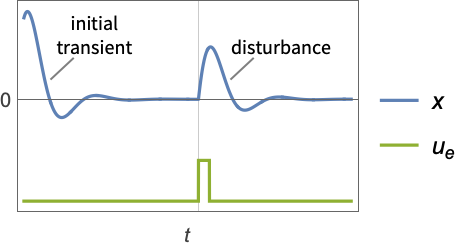
- A regulating controller aims to maintain the system at an equilibrium state despite disturbances
 pushing it away. Typical examples include maintaining an inverted pendulum in its upright position or maintaining an aircraft in level flight.
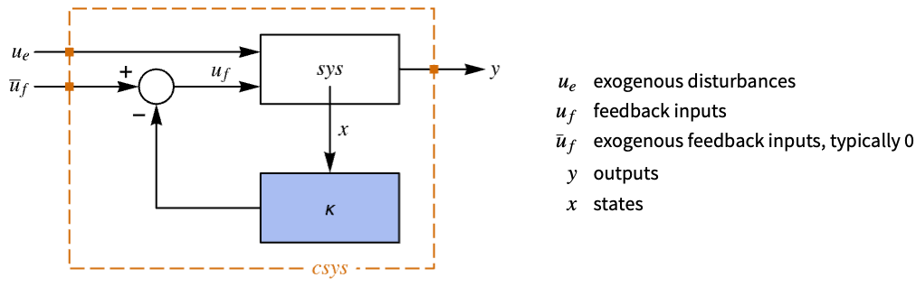
 - The regulating controller is given by a control law of the form
 , where
  is the computed gain matrix.
 - The number of poles n to place is given by SystemsModelOrder of the system sys.
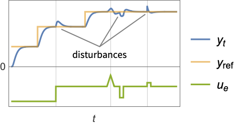
- A tracking controller aims to track a reference signal despite disturbances
 interfering with it. Typical examples include a cruise control system for a car or path tracking for a robot.
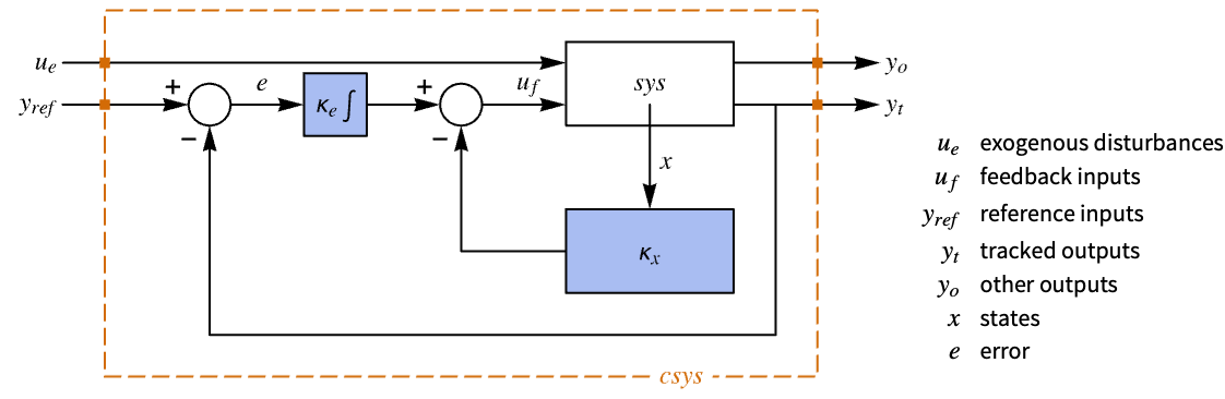
 - The tracking controller is given by a control law of the form
 , where
  is the computed gain matrix for the augmented system that includes the system sys as well as the dynamics for
  .
. - The number of poles n to place is given by
 , where
  is given by SystemsModelOrder of sys,
  the order of yref and
  the number of signals yref.
 - Pole placement works for linear systems as specified by StateSpaceModel:
-

continuous-time system 
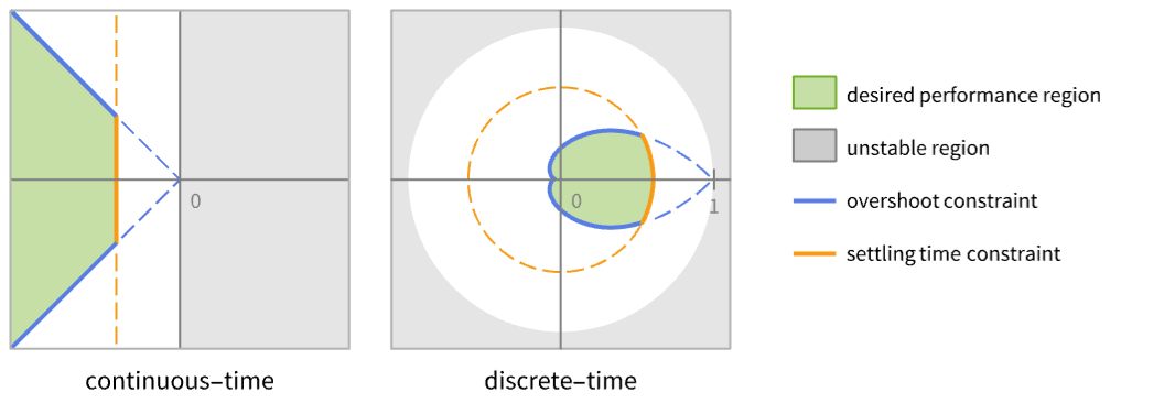
discrete-time system - The performance of the resulting closed-loop system csys is primarily determined by the location of the poles pi.
- Typically there are performance constraints such as settling time and quality constraints such as overshoot. These correspond to certain regions that are desirable pole locations.
- The system specification sspec is the system sys together with the uf, yt and yref specifications.
- The system specification sspec can have the following forms:
-
StateSpaceModel[…] linear control input and linear state AffineStateSpaceModel[…] linear control input and nonlinear state NonlinearStateSpaceModel[…] nonlinear control input and nonlinear state SystemModel[…] general system model <…> detailed system specification given as an Association - The detailed system specification can have the following keys:
-
"InputModel" sys any one of the models "FeedbackInputs" All the feedback inputs uf "TrackedOutputs" None the tracked outputs yt "TrackedSignal" Automatic the dynamics of yref - The tracked signal dynamics is given as a function of the reference signal and time variable. By default, it is assumed to be constant.
-
Function[{r, t},r'[t]] continuous-time system Function[{r,k},r[k+1]-r[k]] discrete-time system - The feedback inputs and tracked outputs can have the following forms:
-
{num1,…,numn} numbered inputs numi used by StateSpaceModel, AffineStateSpaceModel and NonlinearStateSpaceModel {name1,…,namen} named inputs namei used by SystemModel All uses all inputs - For nonlinear systems such as AffineStateSpaceModel, NonlinearStateSpaceModel and SystemModel, the system will be linearized around its stored operating point.
- StateFeedbackGains[…,"Data"] returns a SystemsModelControllerData object cd that can be used to extract additional properties using the form cd["prop"].
- StateFeedbackGains[…,"prop"] can be used to directly get the value of cd["prop"].
- Possible values for properties "prop" include:
-
"BlockDiagram" block diagram of csys {"BlockDiagram",<"SampledData"True>} create a sampled data block diagram of csys "ClosedLoopPoles" poles of the linearized "ClosedLoopSystem" "ClosedLoopSystem" system csys {"ClosedLoopSystem", cspec} detailed control over the form of the closed-loop system "ControllerModel" model cm "Design" type of controller design "DesignModel" model used for the design "FeedbackGains" gain matrix κ or its equivalent "FeedbackGainsModel" model gm or {gm1,gm2} "FeedbackInputs" inputs uf of sys used for feedback "InputModel" input model sys "InputCount" number of inputs u of sys "OpenLoopPoles" poles of "DesignModel" "OutputCount" number of outputs y of sys "SamplingPeriod" sampling period of sys "StateCount" number of states x of sys "TrackedOutputs" outputs yt of sys that are tracked - Possible keys for cspec include:
-
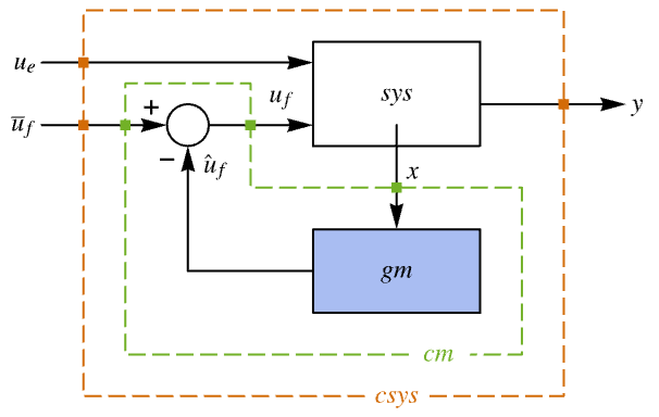
"InputModel" input model in csys "Merge" whether to merge csys "ModelName" name of csys "SamplingPeriod" create a sampled data csys - The diagram of the regulator layout.
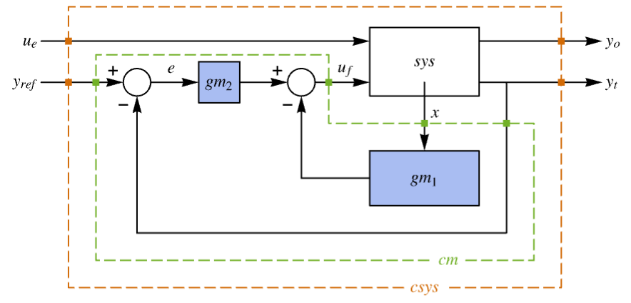
- The diagram of the tracker layout.
- StateFeedbackGains accepts a Method option with settings given by:
-
Automatic automatic method selection "Ackermann" Ackermann method "KNVD" Kautsky–Nichols–Van Dooren method
Examples
open all close allBasic Examples (3)
The feedback gains for a system specification sspec with a feedback uf and exogenous input ue:
sspec = <|"InputModel" -> StateSpaceModel[{{{0, 1}, {1, 2}}, {{1, 0}, {1, 2}}, {{0, 1}}, {{0, 0}}}, SamplingPeriod -> None,
SystemsModelLabels -> {{uf, ue}}], "FeedbackInputs" -> 1|>;p = {-4 + 3I, -4 - 3I};StateFeedbackGains[sspec, p]The feedback gains for a nonlinear system:
nsys = NonlinearStateSpaceModel[{{-1 + Subscript[x, 2],
   u + Subscript[x, 1] - 2*Subscript[x, 2]},
  {Subscript[x, 1] + Subscript[x, 2]}},
 {{Subscript[x, 1], 1}, {Subscript[x, 2], 1}}, {{u, 1}},
 {Automatic}, Automatic, SamplingPeriod -> None];
The gains have an offset because of the nonzero operating points:
p = {-2 + I, -2 - I};StateFeedbackGains[nsys, p]The gains of the approximate linearized system do not have the offset:
StateFeedbackGains[StateSpaceModel[nsys], {-2 + I, -2 - I}]𝒸𝒹 = StateFeedbackGains[StateSpaceModel[{{{0, 5}, {-1, 2.5}}, {{0}, {1}}, {{1, 1}}, {{0}}}, SamplingPeriod -> None,
SystemsModelLabels -> None], {-2, -1.5}, "Data"]Compare the open-loop and closed-loop poles:
PoleZeroPlot[Table[𝒸𝒹[prop], {prop, {"InputModel", "ClosedLoopSystem"}}], IconizedObject[«plotOpts»]]Scope (34)
Basic Uses (8)
Compute the state feedback gain that places the closed-loop pole at p:
ssm = StateSpaceModel[{{{a}}, {{b}}, {{c}}, {{d}}},
SamplingPeriod -> None, SystemsModelLabels -> None];κ = StateFeedbackGains[ssm, {p}]The closed-loop system has pole p:
SystemsModelStateFeedbackConnect[ssm, κ]Compute the gain to stabilize an unstable system:
ssm = StateSpaceModel[{{{2}}, {{1}}, {{1}}, {{0}}}, SamplingPeriod -> None, SystemsModelLabels -> None];κ = StateFeedbackGains[ssm, {-1}]The closed-loop system has pole ![]() :
:
csys = SystemsModelStateFeedbackConnect[ssm, κ]The unstable pole and the stabilized pole can be seen in the system's responses:
Table[Expand[OutputResponse[sys, 1, t]], {sys, {ssm, csys}}];Compute the state feedback gains for a multiple-state system:
ssm = StateSpaceModel[{{{0, 1}, {-1, -2}}, {{0}, {1}}, {{1, 0}}, {{0}}}, SamplingPeriod -> None,
SystemsModelLabels -> None];κ = StateFeedbackGains[ssm, {-2, -3}]The dimensions of the result correspond to the number of inputs and the system's order:
Dimensions[κ]Compute the gains for a system with 2 inputs and 3 states:
ssm = StateSpaceModel[{{{0, 0, -0.1}, {1., 0., -1.08}, {0., 1., -0.9}}, {{1, 1}, {1, 0}, {0, 0}},
{{0, 0, 1}}, {{0, 0}}}, SamplingPeriod -> None, SystemsModelLabels -> None];StateFeedbackGains[ssm, {-1, -2, -2.5}]//MatrixFormPlace the poles at conjugate pole locations:
ssm = StateSpaceModel[{{{0, 1}, {-2, -3}}, {{0}, {1}}, {{2, 0}}, {{0}}}, SamplingPeriod -> None,
SystemsModelLabels -> None];StateFeedbackGains[ssm, {-2 + I , -2 - I}]If the poles are not complex conjugate, the gains will be complex:
StateFeedbackGains[ssm, {-2 , -2 - I}]Place the poles at conjugate pole locations for a multiple-input system:
ssm = StateSpaceModel[{{{0, 0, -0.1}, {1., 0., -1.08}, {0., 1., -0.9}}, {{1, 1}, {1, 0}, {0, 0}},
{{0, 0, 1}}, {{0, 0}}}, SamplingPeriod -> None, SystemsModelLabels -> None];StateFeedbackGains[ssm, {-1 + I , -1 - I, -2}]If the poles are not complex conjugate, the control will be complex and use only one of the inputs:
κ = StateFeedbackGains[ssm, {-1 + I , -1, -2}]The first input is not used for feedback:
Position[κ, {0..}]Choose the feedback inputs for multiple-input systems:
ssm = StateSpaceModel[{{{0, 0, -0.1}, {1., 0., -1.08}, {0., 1., -0.9}}, {{1, 1}, {1, 0}, {0, 0}},
  {{0, 0, 1}}, {{0, 0}}}, SamplingPeriod -> None, SystemsModelLabels -> None];
p = {-1 + I , -1 - I, -2};StateFeedbackGains[<|"InputModel" -> ssm, "FeedbackInputs" -> {1}|>, p]StateFeedbackGains[<|"InputModel" -> ssm, "FeedbackInputs" -> {2}|>, p]StateFeedbackGains[<|"InputModel" -> ssm, "FeedbackInputs" -> {1, 2}|>, p]Compute the gains for a nonlinear system:
assm = AffineStateSpaceModel[{{E^(1 - Subscript[x, 1]) + Subscript[x, 2],
   Subscript[x, 1] - Subscript[x, 2]},
  {{Subscript[x, 1]}, {0}}, {Subscript[x, 1]}, {{0}}},
 {{Subscript[x, 1], 1}, {Subscript[x, 2], 1}}, {{u, -2}},
 {Automatic}, Automatic, SamplingPeriod -> None]
The controller is returned as a vector and takes operating points into consideration:
StateFeedbackGains[assm, {-2, -3}]The controller for the approximate linear system:
StateFeedbackGains[StateSpaceModel[assm], {-2, -3}]Plant Models (6)
Continuous-time StateSpaceModel:
StateFeedbackGains[StateSpaceModel[{{{0, 1.}, {-1, -1.6}}, {{0}, {1}}, {{1, 1}}, {{0}}}, SamplingPeriod -> None,
 SystemsModelLabels -> None], {-1.5 + I, -1.5 - I}]
Discrete-time StateSpaceModel:
StateFeedbackGains[StateSpaceModel[{{{0, 1.}, {0.020000000000000004, 0.1}}, {{0}, {1}}, {{1, 0}}, {{0}}},
 SamplingPeriod -> τ, SystemsModelLabels -> None], {0, 0.1}]
Descriptor StateSpaceModel:
StateFeedbackGains[StateSpaceModel[{{{-6, -4}, {-6, -5}}, {{1}, {1}}, {{1, 0}}, {{0}}, {{1, 1}, {0, 1}}},
 {{x1[t], 0}, {x2[t], 0}},
 {{u[t], 0}}, Automatic, t, SamplingPeriod -> None,
 SystemsModelLabels -> None], {-2.5, -3}]
AffineStateSpaceModel with no operating point is taken to be 0:
StateFeedbackGains[AffineStateSpaceModel[{{Sin[Subscript[x, 1]] + Subscript[x, 2],
   -Subscript[x, 1] - Subscript[x, 2]},
  {{Subscript[x, 1]}, {1}}, {Subscript[x, 1]}, {{0}}},
 {Subscript[x, 1], Subscript[x, 2]}, {{u, 0}}, {Automatic},
 Automatic, SamplingPeriod -> None], {-2, -3}]
NonlinearStateSpaceModel with no operating point is taken to be 0:
StateFeedbackGains[NonlinearStateSpaceModel[
 {{Subscript[x, 2] + Subscript[x, 1]*Subscript[x, 2],
   u + Subscript[x, 1]}, {Subscript[x, 1]}},
 {Subscript[x, 1], Subscript[x, 2]}, {u}, {Automatic},
Automatic, SamplingPeriod -> None], {-1, -2}]sm = CreateSystemModel[{x''[t] + x'[t] + x[t] == 2 u[t], y[t] == x[t]}, t, {"u"∈"Modelica.Blocks.Interfaces.RealInput", "y"∈"Modelica.Blocks.Interfaces.RealOutput"}];StateFeedbackGains[sm, {-1, -2}]Properties (12)
StateFeedbackGains returns the feedback gains by default:
ssm = StateSpaceModel[{{{0, 1}, {-1, -2}}, {{0}, {1}}, {{1, 0}}, {{0}}}, SamplingPeriod -> None,
 SystemsModelLabels -> None];
p = {-2, -3};StateFeedbackGains[ssm, p]% == StateFeedbackGains[ssm, p, "FeedbackGains"]In general, the feedback is affine in the states:
κ = StateFeedbackGains[NonlinearStateSpaceModel[{{f[x, u]},
  {g[x, u]}}, {{x, x0}},
 {{u, u0}}, {Automatic}, Automatic, SamplingPeriod -> None], {p}]
It is of the form κ0+κ1.x, where κ0 and κ1 are constants:
{Subscript[κ, 0], Subscript[κ, 1]} = {κ /. x -> 0, D[κ, {{x}}]}The systems model of the feedback gains:
StateFeedbackGains[StateSpaceModel[{{{0, 1}, {-1, -2}}, {{0}, {1}}, {{1, 0}}, {{0}}}, SamplingPeriod -> None,
 SystemsModelLabels -> None], {-2, -3}, "FeedbackGainsModel"]
An affine feedback gains systems model:
StateFeedbackGains[ NonlinearStateSpaceModel[{{Subscript[x, 2], -2/3 + u -
    Subscript[x, 1]/3 - Subscript[x, 2]/2},
  {Subscript[x, 1]}}, {{Subscript[x, 1], 1},
  {Subscript[x, 2], 0}}, {{u, 1}}, {Automatic}, Automatic,
SamplingPeriod -> None], {-2, -3}, "FeedbackGainsModel"]StateFeedbackGains[StateSpaceModel[{{{0., 1.}, {-0.05, -0.9}}, {{0}, {1}}, {{1, 0}}, {{0}}},
{Subscript[x, 1], Subscript[x, 2]}, {{f, 0}},
SamplingPeriod -> None, SystemsModelLabels -> None], {-1, -2}, "ClosedLoopSystem"]The closed-loop system's block diagram:
StateFeedbackGains[StateSpaceModel[{{{0, 1}, {-1, -2}}, {{0}, {1}}, {{1, 0}}, {{0}}}, SamplingPeriod -> None,
 SystemsModelLabels -> None], {-2, -3}, "BlockDiagram"]
The poles of the linearized closed-loop system:
assm = AffineStateSpaceModel[{{Subscript[x, 2], -0.05*Subscript[x, 1] -
    0.9*Subscript[x, 2]^2}, {{0}, {1}}, {Subscript[x, 1]}, {{0}}},
 {Subscript[x, 1], Subscript[x, 2]}, {{f, 0}}, {Automatic},
 Automatic, SamplingPeriod -> None];
p = {-1, -2};StateFeedbackGains[assm, p, "ClosedLoopPoles"]They should be the specified poles:
ContainsExactly[p, %, SameTest -> (Chop[#1 - #2] == 0 &)]The model used to compute the feedback gains:
assm = AffineStateSpaceModel[{{Subscript[x, 2], -0.05*Subscript[x, 1] -
    0.9*Subscript[x, 2]^2}, {{0}, {1}}, {Subscript[x, 1]}, {{0}}},
 {Subscript[x, 1], Subscript[x, 2]}, {{f, 0}}, {Automatic},
 Automatic, SamplingPeriod -> None];
p = {-1, -2};Subscript[ssm, 𝒟] = StateFeedbackGains[assm, p, "DesignModel"]The feedback gains of the input model and the design model, respectively:
Table[{StateFeedbackGains[s, p]}, {s, {assm, Subscript[ssm, 𝒟]}}]StateFeedbackGains[AffineStateSpaceModel[{{Subscript[x, 2], -0.05*Subscript[x, 1] -
0.9*Subscript[x, 2]^2}, {{0}, {1}}, {Subscript[x, 1]}, {{0}}},
{Subscript[x, 1], Subscript[x, 2]}, {{f, 0}}, {Automatic},
Automatic, SamplingPeriod -> None], {-1, -2}, "Design"]StateFeedbackGains[StateSpaceModel[{{{0, 1}, {-1, -2}}, {{0}, {1}}, {{1, 0}}, {{0}}}, SamplingPeriod -> None,
SystemsModelLabels -> None], {-2, -3}, "Data"]Properties related to the input model:
Dataset[Table[{prop, StateFeedbackGains[IconizedObject[«sys»], IconizedObject[«p»], prop]}, {prop, IconizedObject[«props»]}]]Get the controller data object:
𝒸𝒹 = StateFeedbackGains[IconizedObject[«sys»], IconizedObject[«p»], "Data"]The list of available properties:
𝒸𝒹["Properties"]The value of a specific property:
𝒸𝒹["ClosedLoopPoles"]Tracking (5)
sspec = <|"InputModel" -> StateSpaceModel[{{{0, 1}, {-3, -4}}, {{0}, {1}}, {{3, 0}}, {{0}}}, SamplingPeriod -> None,
SystemsModelLabels -> None], "TrackedOutputs" -> 1|>;𝒸𝒹 = StateFeedbackGains[sspec, {-3.5, -2 + 0.8I, -2 - 0.8I}, "Data"]The closed-loop system tracks the reference signal ![]() :
:
OutputResponse[𝒸𝒹["ClosedLoopSystem"], 1, {t, 0, 5}];
Plot[{1, %}, {t, 0, 5}, IconizedObject[«plotOpts»]]
The block diagram of the closed-loop system:
𝒸𝒹["BlockDiagram"]Design a tracking controller for a discrete-time system:
sspec = <|"InputModel" -> StateSpaceModel[{{{0, 1.}, {0.2, -1.9}}, {{0}, {1}}, {{1, 0}}, {{0}}}, SamplingPeriod -> 1,
SystemsModelLabels -> None], "TrackedOutputs" -> 1|>;𝒸𝒹 = StateFeedbackGains[sspec, {0.6, -0.1 + 0.1I, -0.1 - 0.1I}, "Data"]The closed-loop system tracks the reference signal ![]() :
:
ref = Table[1, 15];
OutputResponse[𝒸𝒹["ClosedLoopSystem"], ref];ListLinePlot[{ref, %[[1]]}, IconizedObject[«plotOpts»]]sspec = <|"InputModel" -> StateSpaceModel[{{{1, 0}, {2, -1}}, {{1, 0}, {1, 1}}, {{1, 0}, {1, 1}}, {{0, 0}, {0, 0}}},
SamplingPeriod -> None, SystemsModelLabels -> None], "TrackedOutputs" -> {1, 2}|>;𝒸𝒹 = StateFeedbackGains[sspec, {-2, -3, -1 + I, -1 - I}//N, "Data"]The closed-loop system tracks two different reference signals:
refs = RandomInteger[{-7, -1}, 2];
or = OutputResponse[𝒸𝒹["ClosedLoopSystem"], refs, {t, 0, 10}];Plot[Evaluate[Riffle[refs, or]], {t, 0, 10}, IconizedObject[«plotOpts»]]Compute the controller effort:
sspec = <|"InputModel" -> StateSpaceModel[{{{0, 1}, {-3, -4}}, {{0}, {1}}, {{3, 0}}, {{0}}}, SamplingPeriod -> None,
SystemsModelLabels -> None], "TrackedOutputs" -> 1|>;𝒸𝒹 = StateFeedbackGains[sspec, {-3.5, -2 + 0.8I, -2 - 0.8I}, "Data"]cm = 𝒸𝒹["ControllerModel"]ref = {1};
csys = 𝒸𝒹["ClosedLoopSystem"];
n = SystemsModelOrder[sspec["InputModel"]];cinps = Join[ref, OutputResponse[csys, ref, {t, 0, 5}], StateResponse[csys, ref, {t, 0, 5}][[1 ;; n]]]OutputResponse[cm, cinps, {t, 0, 5}];
Plot[%, {t, 0, 5}, PlotRange -> All]Track a desired reference signal:
tSig = Function[{r, t}, r''[t] + r[t]]The reference signal is of order 2:
m = Max[Join[Cases[tSig[r, t], Derivative[n_][r][t] :> n], {0}]]ref = r[t] /. DSolve[Join[{tSig[r, t] == 0}, {r[0] == 0, r'[0] == 1}], r[t], t]Design a controller to track one output of a first-order system:
sspec = <|"InputModel" -> StateSpaceModel[{{{-1}}, {{1}}, {{1}}, {{0}}}, SamplingPeriod -> None, SystemsModelLabels -> None], "TrackedOutputs" -> {1}, "TrackedSignal" -> tSig|>;{q, k} = {Length[sspec["TrackedOutputs"]], SystemsModelOrder[sspec["InputModel"]]}The number of pole specifications is k+m q:
p = {-2, -1.5 + 0.8I, -1.5 - 0.8I};
Length[p] == k + m q𝒸𝒹 = StateFeedbackGains[sspec, p, "Data"]The closed-loop system tracks the reference:
OutputResponse[𝒸𝒹["ClosedLoopSystem"], ref, {t, 0, 10}];
Plot[{ref, %}, {t, 0, 10}, IconizedObject[«plotOpts»]]
Closed-Loop System (3)
Assemble the closed-loop system for a nonlinear plant model:
assm = AffineStateSpaceModel[{{Subscript[x, 1] + Subscript[x, 2],
   -Subscript[x, 1]^3 - Subscript[x, 2]}, {{0}, {1}},
  {Subscript[x, 1]}, {{0}}}, {Subscript[x, 1],
Subscript[x, 2]}, {u}, {Automatic}, Automatic, SamplingPeriod -> None];Subscript[csys, 1] = StateFeedbackGains[assm, {-2, -3}, "ClosedLoopSystem"]The closed-loop system with a linearized model:
Subscript[csys, 2] = StateFeedbackGains[StateSpaceModel[assm], {-1, -2}, "ClosedLoopSystem"]Compare the response of the two systems:
Table[OutputResponse[{sys, {0.5, 1}}, 0, {t, 0, 7}], {sys, {Subscript[csys, 1], Subscript[csys, 2]}}];
Plot[%, {t, 0, 7}, PlotLegends -> {"Nonlinear", "Linear"}, PlotRange -> All]
Assemble the merged closed-loop of a plant with one disturbance and one feedback input:
sys = <|"InputModel" -> StateSpaceModel[{{{0., 1.}, {-0.05, -0.9}}, {{0, 0}, {1, 1}}, {{1, 0}}, {{0, 0}}},
 {Subscript[x, 1], Subscript[x, 2]},
 {{d, 0}, {f, 0}}, SamplingPeriod -> None,
 SystemsModelLabels -> {{Subscript[u, e],
    Subscript[u, f]}}], "FeedbackInputs" -> 2|>;
p = {-1, -2};StateFeedbackGains[sys, p, "ClosedLoopSystem"]The unmerged closed-loop system:
StateFeedbackGains[sys, p, {"ClosedLoopSystem", <|"Merge" -> False|>}]When merged, it gives the same result as before:
SystemsModelMerge[%]Explicitly specify the merged closed-loop system:
StateFeedbackGains[sys, p, {"ClosedLoopSystem", <|"Merge" -> True|>}]Create a closed-loop system with a desired name:
sm = CreateSystemModel["MassSpringDamper", {m x''[t] + c x'[t] + k x[t] == u[t], y[t] == x[t]}, t, {"u"∈"Modelica.Blocks.Interfaces.RealInput", "y"∈"Modelica.Blocks.Interfaces.RealOutput"}, <|"ParameterValues" -> {m -> 10, c -> 10^2, k -> 10^3}|>];csysName = "MassSpringDamperWithStateFeedback";csys = StateFeedbackGains[sm, {-2, -3}, {"ClosedLoopSystem", <|"ModelName" -> csysName|>}]The closed-loop system has the specified name:
csys["ModelName"]The name can be directly used to specify the closed-loop model in other functions:
SystemModelSimulate[csysName, {"y"}, 10, <|"Inputs" -> {"u" -> UnitStep}|>]SystemModelPlot[%, All]Options (6)
Method (6)
The "Ackermann" method is used by default for systems with exact or symbolic values:
ssm = StateSpaceModel[{{{0, 1}, {-k/m, -c/m}},
  {{c/m}, {-c^2/m^2 +
     k/m}}, {{1, 0}}, {{0}}}, SamplingPeriod -> None,
 SystemsModelLabels -> None];
StateFeedbackGains[ssm, {Subscript[p, 1], Subscript[p, 2]}]StateFeedbackGains[ssm, {Subscript[p, 1], Subscript[p, 2]}, Method -> "Ackermann"] === %The "KNVD" method is used by default for inexact systems:
ssm = StateSpaceModel[{{{-1.2, 0.2}, {1., -4.1}}, {{2., 0}, {0., 1.}}, {{1., 1.1}}, {{0, 0}}},
 SamplingPeriod -> None, SystemsModelLabels -> None];
StateFeedbackGains[ssm, {-1., -2.}]StateFeedbackGains[ssm, {-1., -2.}, Method -> "KNVD"] === %LinearSolve is used for inexact systems with at least as many inputs as states:
StateFeedbackGains[StateSpaceModel[{{{a}}, {{Subscript[b, 1],
    Subscript[b, 2]}}, {{c}}, {{0, 0}}}, SamplingPeriod -> None,
SystemsModelLabels -> None], {p}, Method -> Automatic]LinearSolve[{{Subscript[b, 1], Subscript[b, 2]}}, {{a - p}}]The "KNVD" method is typically used for multi-input systems:
ssm = StateSpaceModel[{{{-1.2, 0.2}, {1., -4.1}}, {{2., 0}, {0., 1.}}, {{1., 1.1}}, {{0, 0}}},
 SamplingPeriod -> None, SystemsModelLabels -> None];
p = {-3 + 2 I, -3 - 2I };StateFeedbackGains[ssm, p] === StateFeedbackGains[ssm, p, Method -> "KNVD"]The "Ackermann" method uses only one input for multi-input systems:
ssm = StateSpaceModel[{{{-1.2, 0.2}, {1., -4.1}}, {{2., 0}, {0., 1.}}, {{1., 1.1}}, {{0, 0}}},
 SamplingPeriod -> None, SystemsModelLabels -> None];
p = {-3 + 2 I, -3 - 2I };κ = StateFeedbackGains[ssm, p, Method -> "Ackermann"]Position[κ, {0..}]The input selected has the lowest controllability matrix condition number:
Table[SingularValueList[ControllabilityMatrix[SystemsModelExtract[ssm, i]]], {i, 2}];Table[i[[1]] / i[[-1]], {i, %}]The "KNVD" closed-loop poles are less sensitive to the feedback gain perturbations than "Ackermann":
ssm = StateSpaceModel[{{{-10, 0, -10, 0}, {0, -0.7, 9, 0}, {0, -1, -0.7, 0}, {1, 0, 0, 0}},
  {{20, 2.8}, {0, -3.13}, {0, 0}, {0, 0}}}, SamplingPeriod -> None, SystemsModelLabels -> None];
p = {-10, -8, -5, -2};MatrixForm /@ {Subscript[κ, 1] = StateFeedbackGains[ssm, p, Method -> "KNVD"], Subscript[κ, 2] = StateFeedbackGains[ssm, p, Method -> "Ackermann"]}Add random perturbations to the gain matrices:
δp = RandomReal[{-0.1, 0.1}, Dimensions[Subscript[κ, 1]]];
MatrixForm /@ {Subscript[κ, 1] += δp, Subscript[κ, 2] += δp}
The resulting closed-loop poles:
csys = Table[SystemsModelStateFeedbackConnect[ssm, κ], {κ, {Subscript[κ, 1], Subscript[κ, 2]}}];
{Subscript[p, 1], Subscript[p, 2]} = Table[Eigenvalues@First@Normal[sys], {sys, csys}]
The maximum error from the specified poles is smaller for the "KNVD" method:
Table[Norm[(pl - p/p), Infinity], {pl, {Subscript[p, 1], Subscript[p, 2]}}]Applications (14)
Mechanical Systems (4)
Design a balancing controller for a Segway PT:
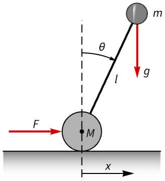
A nonlinear model of the Segway PT:
segw = NonlinearStateSpaceModel[IconizedObject[«eqns»] /. IconizedObject[«pars»], {x[t], x'[t], {θ[t], 0}, θ'[t]}, f[t], {x[t], θ[t]}, t]//SimplifyWithout a controller, the Segway's position and orientation are not balanced:
OutputResponse[{segw, {0, 0, 0.1}}, 0, {t, 0, 10}];
Plot[%, {t, 0, 10}, PlotRange -> All, PlotLegends -> {θ, x}]
Design a controller to balance the Segway using pole placement:
segw = NonlinearStateSpaceModel[segw, Automatic, Automatic, Automatic, None];p = {-2 + 0.5I, -2 - 0.5I, -3.5, -1.5};
𝒸𝒹 = StateFeedbackGains[segw, p, "Data"]𝒸𝒹["ClosedLoopPoles"]The open-loop system was unstable:
𝒸𝒹["OpenLoopPoles"]Obtain the closed-loop system:
csys = 𝒸𝒹["ClosedLoopSystem"]//FullSimplifyIt is balanced from a nonzero initial position:
sr = StateResponse[{csys, {0, 0, 0.1}}, 0, {t, 0, 10}];
Table[Plot[𝓈𝓇[[1]], {t, 0, 15}, IconizedObject[«plotOpts»]], {𝓈𝓇, ({sr, {θ, ω, x, x'}})}]So is its response to a nudge:
or = OutputResponse[csys, 0.2UnitBox[t - 1], {t, 0, 20}];
Table[Plot[ℴ𝓇[[1]], {t, 0, 15}, IconizedObject[«plotOpts»]], {ℴ𝓇, ({or, {θ, x}})}]OutputResponse[𝒸𝒹["ControllerModel"], Join[{0}, sr], {t, 0, 10}];
Plot[%, {t, 0, 10}, PlotRange -> All]Design a regulator for a single-link robotic manipulator with a flexible joint:
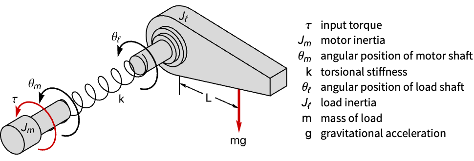
robotM = NonlinearStateSpaceModel[IconizedObject[«eqns»] /. IconizedObject[«pars»], {θ[t], θ'[t], ϕ[t], ϕ'[t]}, τ[t], θ[t], t];
robotM = NonlinearStateSpaceModel[robotM, Automatic, Automatic, Automatic, None]
The arm's angular position is unregulated:
OutputResponse[{robotM, {0.2}}, 0, {t, 0, 15}];
Plot[%, {t, 0, 15}, PlotRange -> All]
Design a state feedback controller:
p = {-1 + I, -1 - I, -4 + 0.25I, -4 - 0.25I};
𝒸𝒹 = StateFeedbackGains[robotM, p, "Data"]
Obtain the closed-loop system:
csys = 𝒸𝒹["ClosedLoopSystem"]The feedback controller regulates the arm's angular position:
sr = StateResponse[{csys, {0.05}}, 0, {t, 0, 15}];
Table[Plot[𝓈𝓇[[1]], {t, 0, 15}, IconizedObject[«plotOpts»]], {𝓈𝓇, ({sr, {θ, θ', ϕ, ϕ'}})}]cm = 𝒸𝒹["ControllerModel"]OutputResponse[cm, Join[{0}, sr], {t, 0, 10}];
Plot[%, {t, 0, 10}, PlotRange -> All]Design a discrete-time stabilizing controller for a ball and beam system:
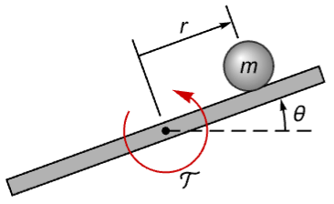
A linear continuous-time model of the system:
bbs = StateSpaceModel[IconizedObject[«eqns»] /. IconizedObject[«pars»], {r[t], θ[t]}, 𝒯[t], r[t], t, IconizedObject[«labels»]]Discretize the model with a sampling period of ![]() :
:
τ = 0.2;
bbd = ToDiscreteTimeModel[bbs, τ]
The ball's position is unstable if the beam is perturbed:
OutputResponse[{bbd, {0, 0, 0.01}}, Table[0, 10]];
ListStepPlot[%, DataRange -> {0, 9 τ}, PlotRange -> All]
Compute a stabilizing controller:
p = {0.7, -0.75, 0.05 + 0.0125I, 0.05 - 0.0125I};
𝒸𝒹 = StateFeedbackGains[bbd, p, "Data"]
Obtain the closed-loop system:
csys = 𝒸𝒹["ClosedLoopSystem"]The ball's position is stabilized:
sr = StateResponse[{csys, {0, 0, 0.25, 0}}, Table[0, 30]];
ListStepPlot[%[[1]], DataRange -> {0, 29 τ}, PlotRange -> All]OutputResponse[𝒸𝒹["ControllerModel"], Join[{Table[0, 30]}, sr]];
ListStepPlot[%, DataRange -> {0, 29 τ}, PlotRange -> All]Suppress the oscillations of a two-mass damper system:
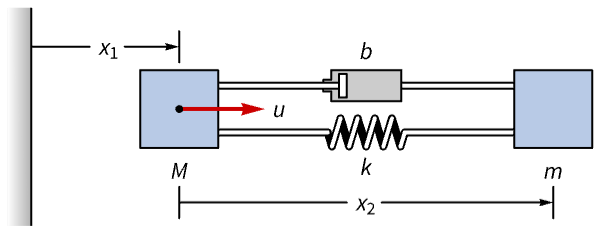
ssm = StateSpaceModel[IconizedObject[«eqns»] /. IconizedObject[«pars»], {Subscript[x, 1][t], Subscript[x, 1]'[t], Subscript[x, 2][t], Subscript[x, 2]'[t]}, u[t], {Subscript[x, 1][t], Subscript[x, 2][t]}, t, IconizedObject[«labels»]]Discretize it with a sampling period of ![]() using the zero-order hold method:
using the zero-order hold method:
τ = 0.4;
ssmd = ToDiscreteTimeModel[ssm, 0.4, Method -> "ZeroOrderHold"]
The masses ![]() and
and ![]() oscillate when perturbed:
oscillate when perturbed:
OutputResponse[{ssmd, {1}}, Table[0, 30]];
ListStepPlot[%, DataRange -> {0, 29 τ}, IconizedObject[«plotOpts»]]
Compute state feedback gains for a set of poles within the unit circle:
Subscript[𝒸𝒹, 1] = StateFeedbackGains[ssmd, {0.9, 0.4, 0.3, 0.1}, "Data"]Compute gains for a set of poles that are less damped:
Subscript[𝒸𝒹, 2] = StateFeedbackGains[ssmd, {0.75 + 0.4I, 0.75 - 0.4I, 0.1, 0.2}, "Data"]Obtain the closed-loop systems for each set of poles:
{Subscript[csys, 1], Subscript[csys, 2]} = Table[Subscript[𝒸𝒹, i]["ClosedLoopSystem"], {i, 2}]Compare their responses to a perturbation:
{Subscript[sr, 1], Subscript[sr, 2]} = Table[StateResponse[{Subscript[csys, i], {1}}, Table[0, 30]], {i, 2}];Table[ListStepPlot[Subscript[sr, i][[{1, 3}]], DataRange -> {0, 29τ}, IconizedObject[«plotOpts»]], {i, 2}]{Subscript[κ, 1], Subscript[κ, 2]} = Table[Subscript[𝒸𝒹, i]["FeedbackGains"], {i, 2}]Compare their control efforts:
Table[ListStepPlot[-Subscript[κ, i].Subscript[sr, i], PlotRange -> All, ImageSize -> Small], {i, 2}]Electromechanical Systems (1)
Dampen the oscillations on an angular gauge:
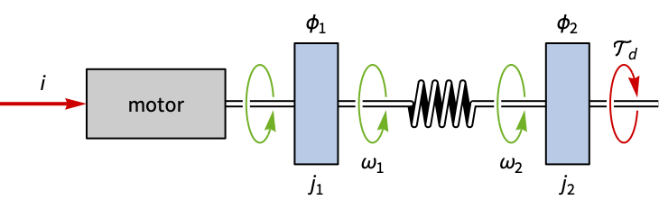
gauge = StateSpaceModel[IconizedObject[«eqns»] /. IconizedObject[«pars»], {Subscript[ϕ, 1][t], Subscript[ω, 1][t], Subscript[ϕ, 2][t], Subscript[ω, 2][t]}, {i[t] , Subscript[𝒯, d][t]}, Subscript[ϕ, 2][t], t, IconizedObject[«labels»]]A disturbance of the gauge's position results in significant oscillations:
OutputResponse[{gauge, {0.1, 0, -0.1}}, {0, 0}, {t, 0, 200}];
Plot[%, {t, 0, 200}, PlotRange -> All]
Set the current i as the feedback input:
sspec = <|"InputModel" -> gauge, "FeedbackInputs" -> 1|>;Design a state feedback controller to dampen the oscillations:
p = {-2, -1.5, -1 + I, -1 - I};
𝒸𝒹 = StateFeedbackGains[sspec, p, "Data"]𝒸𝒹["ClosedLoopPoles"]Obtain the closed-loop system:
csys = 𝒸𝒹["ClosedLoopSystem"]sr = StateResponse[{csys, {0.1, 0, -0.1}}, {0, 0}, {t, 0, 10}];
Plot[%[[4]], {t, 0, 10}, PlotRange -> All]A sinusoidal torque disturbance is also blocked by the controller:
OutputResponse[csys, {0, 0.1Sin[t]}, {t, 0, 100}];
Plot[%, {t, 0, 100}, PlotRange -> {1, -1}]cm = 𝒸𝒹["ControllerModel"]OutputResponse[cm, Join[{0}, sr], {t, 0, 10}];
Plot[%, {t, 0, 10}, IconizedObject[«plotOpts»]]Aerospace Systems (2)
Improve the handling of an aircraft's response about the longitudinal axis:
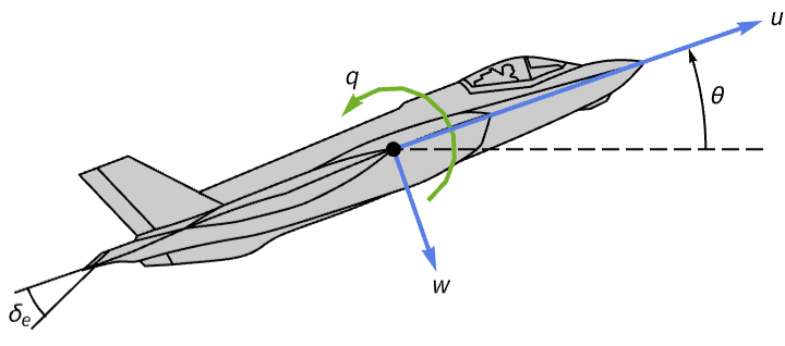
aircraft = NonlinearStateSpaceModel[IconizedObject[«eqns»] /. IconizedObject[«pars»], {u[t], w[t], q[t], θ[t]}, Subscript[δ, e][t], θ[t], t]Its pitch angle takes about 1500 seconds to stabilize after an initial perturbation:
OutputResponse[{aircraft, {0, 0, 0, 0.1}}, 0, {t, 0, 2000}];
Plot[%, {t, 0, 2000}, PlotRange -> All]
Design a controller to improve the response:
aircraft = NonlinearStateSpaceModel[aircraft, Automatic, Automatic, Automatic, None];p = {-3, -1 + 0.5I, -1 - 0.5I, -1};
𝒸𝒹 = StateFeedbackGains[aircraft, p, "Data"]Obtain the closed-loop system:
csys = 𝒸𝒹["ClosedLoopSystem"]The response of the closed-loop system now stabilizes in about 10 seconds:
sr = StateResponse[{csys, {0, 0, 0, 0.1}}, 0, {t, 0, 15}];
Table[Plot[𝓈𝓇[[1]], {t, 0, 15}, IconizedObject[«plotOpts»]], {𝓈𝓇, ({sr, {u, w, q, θ}})}]cm = 𝒸𝒹["ControllerModel"]OutputResponse[cm, Join[{0}, sr], {t, 0, 20}];Plot[%, {t, 0, 5}, PlotRange -> All]Design an output feedback controller to regulate an orbiting satellite's trajectory:

sat = StateSpaceModel[IconizedObject[«eqns»] /. ω -> 0.0011, {x[t], x'[t], y[t], y'[t]}, {Subscript[f, x][t], Subscript[f, y][t]}, {x[t], y[t]}, t, IconizedObject[«labels»]]The orbit is unstable if perturbed:
OutputResponse[{sat, {0, 0.2, 0, 0.1}}, {0, 0}, {t, 0, 10}];
Table[Plot[%[[i]], {t, 0, 10}, IconizedObject[«plotOpts»]], {i, 2}]
Compute a set of feedback gains:
MatrixForm[κ = StateFeedbackGains[sat, {-0.5, -1.5, -1, -2.5}]]Compute a set of estimator gains:
MatrixForm[ℓ = EstimatorGains[sat, 3 {-0.5, -1.5, -1, -2.5}]]Assemble the estimator regulator:
ℯ𝓇 = EstimatorRegulator[sat, {ℓ, κ}, "Data"]Obtain the closed-loop system:
csys = ℯ𝓇["ClosedLoopSystem"]//SystemsModelMergeCompute the response of the closed-loop system:
or = OutputResponse[{csys, {0, 0.2, 0, 0.1}}, {0, 0}, {t, 0, 15}];
Plot[or, {t, 0, 15}, IconizedObject[«plotOpts»]]cm = ℯ𝓇["ControllerModel"]//SystemsModelMergeOutputResponse[cm, Join[{0}, or], {t, 0, 15}];
Plot[%, {t, 0, 15}, IconizedObject[«plotOpts»]]Electrical Systems (3)
Tune the frequency response of a circuit:

A descriptor model of the circuit:
circuit = StateSpaceModel[Join[IconizedObject[«comps»], IconizedObject[«eqns»]], IconizedObject[«vars»], Subscript[v, s][t], Subscript[v, c2][t],
	t, DescriptorStateSpace -> True, IconizedObject[«labels»]] /. IconizedObject[«pars»]
Its step response is highly oscillatory:
OutputResponse[circuit, UnitStep[t], {t, 0, 10}];
Plot[%, {t, 0, 10}, PlotRange -> All, ImageSize -> Small]
The oscillatory response is due to its underdamped poles:
TransferFunctionPoles@TransferFunctionModel[circuit]//NDesign a state feedback controller with poles that are not underdamped:
p = {-2, -5 + I, -5 - 1I};
𝒸𝒹 = StateFeedbackGains[circuit, p, "Data"]
Obtain the closed-loop system:
csys = 𝒸𝒹["ClosedLoopSystem"]//SystemsModelMergesr = StateResponse[csys, UnitStep[t], {t, 0, 10}];
Plot[%[[2]], {t, 0, 10}, PlotRange -> All]Compare the frequency responses of the open- and closed-loop systems:
BodePlot[{circuit, csys}, IconizedObject[«plotOpts»]]Plot[-𝒸𝒹["FeedbackGains"].sr, {t, 0, 10}, PlotRange -> All]Tune an active bandpass filter:
tfm = BiquadraticFilterModel[{"Bandpass", {{60, 5}}}, s]A state-space realization of the filter:
filter = StateSpaceModel[tfm]TransferFunctionPoles[tfm][[1, 1]]//NDesign a set of controllers to improve the filter's characteristics:
p = {{-6 + 50I, -6 - 50I}, {-15 + 40I, -15 - 40I}, {-25 + 30I, -25 - 30I}};
csys = Table[StateFeedbackGains[filter, 𝓅, "ClosedLoopSystem"], {𝓅, p}]
The more damped the poles are, the smaller the oscillations:
or = Table[OutputResponse[sys, Sin[t], {t, 0, 2}], {sys, Join[{filter}, csys]}];
Table[Plot[ℴ𝓇[[1]], {t, 0, 2}, IconizedObject[«plotOpts»]], {ℴ𝓇, ({or, IconizedObject[«plotLabels»]})}]Design a speed controller for a DC motor:
dcMot = StateSpaceModel[TransferFunctionModel[{{{100.23330719585297}}, 1 + 0.8*s}, s], SystemsModelLabels -> {"v", "ω"}]Set the motor speed as a tracked output:
sspec = <|"InputModel" -> dcMot, "TrackedOutputs" -> 1|>Compute a pole placement controller:
𝒸𝒹 = StateFeedbackGains[sspec, {-1.5, -2}, "Data"]ℓ = EstimatorGains[sspec, {-3}]Assemble an estimator regulator that tracks the motor velocity:
ℯ𝓇 = EstimatorRegulator[sspec, {ℓ, 𝒸𝒹}, "Data"]csys = ℯ𝓇["ClosedLoopSystem"]The response to a reference speed of ![]() rpm:
rpm:
ref = 200;
or = OutputResponse[csys, ref, {t, 0, 7}];Plot[{or, ref}, {t, 0, 7}, IconizedObject[«plotOpts»]]OutputResponse[ℯ𝓇["ControllerModel"], {ref, or[[1]]}, {t, 0, 5}]Plot[%, {t, 0, 5}, PlotRange -> All]Chemical Systems (2)
Improve the response of the flow rate in a mixing tank:
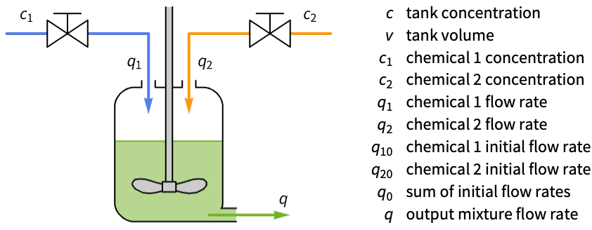
ssm = StateSpaceModel[IconizedObject[«eqns»], IconizedObject[«vars»], IconizedObject[«labels»], DescriptorStateSpace -> True] /. Subscript[q, 0] -> Subscript[q, 10] + Subscript[q, 20] /. IconizedObject[«pars»]The response to a disturbance in the flow rate q2 is sluggish:
olor = OutputResponse[ssm, {0, UnitBox[t - 1]}, {t, 0, 300}];
Plot[olor, {t, 0, 300}, PlotRange -> All]
Design a state feedback controller to accelerate the response:
𝒸𝒹 = StateFeedbackGains[ssm, {-0.5, -0.3}, "Data"]csys = 𝒸𝒹["ClosedLoopSystem"]//ChopThe response of the closed-loop system is faster:
clsr = StateResponse[csys, {0, UnitBox[t - 1]}, {t, 0, 300}];
Plot[{olor, clsr[[3]]}, {t, 0, 300}, IconizedObject[«plotOpts»]]κ = 𝒸𝒹["FeedbackGains"]Plot[Evaluate[-κ.clsr], {t, 0, 50}, IconizedObject[«plotOpts»]]Improve the response of a two-stage chemical reactor with delayed recycle:
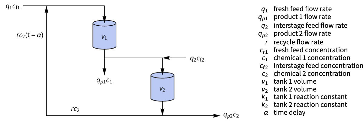
reactor = StateSpaceModel[IconizedObject[«eqns»], {Subscript[c, 1][t], Subscript[c, 2][t]}, {Subscript[c, f1][t], Subscript[c, f2][t]},
	{Subscript[c, 1][t - Subscript[τ, 1]], Subscript[c, 2][t - Subscript[τ, 2]]}, t, IconizedObject[«labels»]] /. IconizedObject[«pars»]
The reactor's response to a perturbation is delayed:
OutputResponse[{reactor, {0.1, -0.1}}, {0, 0}, {t, 0, 10}];
Plot[%, {t, 0, 10}, IconizedObject[«plotOpts»]]
Remove the delay and obtain a minimal realization of the model:
dfsys = MinimalStateSpaceModel[SystemsModelDelayApproximate[reactor, 0]]Compute a set of regulator gains:
κ = StateFeedbackGains[dfsys, {-3 + I, -3 - I}]ℓ = EstimatorGains[dfsys, {-5, -6}]Assemble the estimator regulator using the computed gains:
ℯ𝓇𝒻𝒷 = EstimatorRegulator[dfsys, {ℓ, κ}, "EstimatorRegulatorFeedbackModel"]Assemble a Smith compensator for the original system:
smC = SmithDelayCompensator[reactor, ℯ𝓇𝒻𝒷]Obtain the closed-loop system of the model with the Smith compensator in the feedback path:
csys = SystemsModelFeedbackConnect[SystemsModelSeriesConnect[smC, reactor]]The closed-loop response to an initial perturbation has been improved:
OutputResponse[{csys, {0.1, -0.1}}, {0, 0}, {t, 0, 10}];
Plot[%, {t, 0, 10}, IconizedObject[«plotOpts»]]
Deadbeat Control (1)
Solve the deadbeat control problem for a discrete-time system:
dssm = StateSpaceModel[{{{1, 1, -2}, {0, 1, 1}, {0, 0, 1}}, {{1}, {0}, {1}}}, SamplingPeriod -> 1,
 SystemsModelLabels -> None];
The closed-loop system with all poles at the origin:
csys = StateFeedbackGains[dssm, {0, 0, 0}, "ClosedLoopSystem"]The order of the open-loop system is ![]() :
:
SystemsModelOrder[dssm]Thus the closed-loop system's outputs are zero within three steps:
or = OutputResponse[{csys, RandomReal[{-1, 1}, 3]}, Table[0, 6]]//ChopListStepPlot[or, Right, PlotRange -> All, DataRange -> {0, 5}]Nautical Systems (1)
Design a controller for a boat to track a desired heading angle:
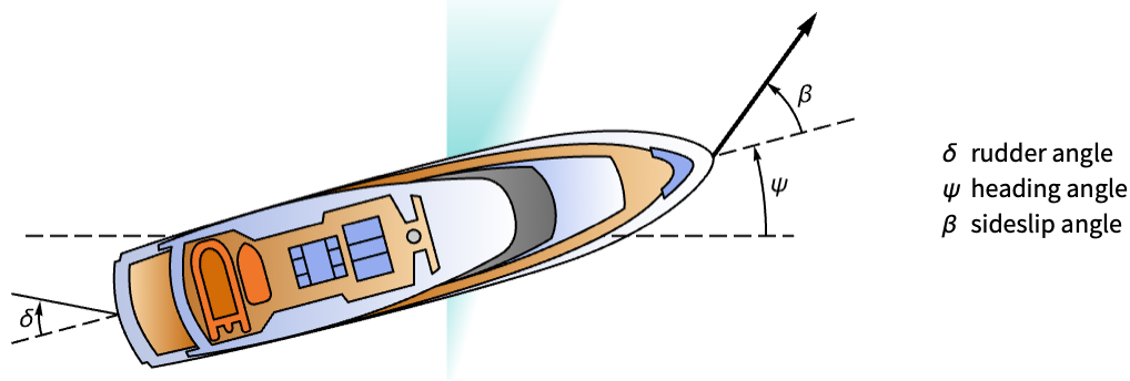
boat = StateSpaceModel[IconizedObject[«abc»], IconizedObject[«labels»]]Design a tracking controller with poles at the desired locations:
sspec = <|"InputModel" -> boat, "TrackedOutputs" -> 1|>;cd = StateFeedbackGains[sspec, {-0.35, -0.3, -0.25 + 0.1I, -0.25 - 0.1I}, "Data"]csys = cd["ClosedLoopSystem"]The response for various heading angle references:
Table[OutputResponse[csys, ref, {t, 0, 50}], {ref, 4, 20, 4}];
Plot[%, {t, 0, 50}, IconizedObject[«plotOpts»]]cm = cd["ControllerModel"]cinps[ref_] := Join[{ref}, OutputResponse[csys, ref, {t, 0, 50}], StateResponse[csys, ref, {t, 0, 50}][[1 ;; 3]]]The control effort increases as the reference value increases:
Table[OutputResponse[cm, cinps[ref], {t, 0, 50}], {ref, 4, 20, 4}];
Plot[%, {t, 0, 50}, IconizedObject[«plotOpts»]]
Properties & Relations (17)
The state feedback gains are computed for negative feedback:
a = RandomReal[{-1, 1}, {2, 2}];
b = RandomReal[{-1, 1}, {2, 1}];
p = RandomReal[{-3, -1}, 2];κ = StateFeedbackGains[StateSpaceModel[{a, b}], p]The closed-loop poles with negative feedback -κ.x:
p1 = Eigenvalues[a - b.κ]They are the same as the specified poles:
ContainsExactly[p1, p, SameTest -> (Chop[#1 - #2] == 0. &)]The closed-loop system is obtained using state feedback:
𝒸𝒹 = StateFeedbackGains[StateSpaceModel[{{{-1, 2}, {1, 3}}, {{1}, {0}}, {{1, 0}}, {{0}}}, SamplingPeriod -> None,
SystemsModelLabels -> None], {-3, -4}, "Data"]SystemsModelStateFeedbackConnect[𝒸𝒹["InputModel"], 𝒸𝒹["FeedbackGains"]]Obtain it directly as a property:
𝒸𝒹["ClosedLoopSystem"]The control effort increases as the closed-loop poles are moved farther away from the open-loop poles:
ssm = StateSpaceModel[{{{-3, 0}, {0, -2}}, {{1}, {-1}}}, SamplingPeriod -> None,
 SystemsModelLabels -> None];
p = {{-3, -2}, {-3, -2.5}, {-2.5, -2}, {-4, -1}, {-4, -5}};ListLinePlot[Table[{Norm[𝓅 - {-3, -2}], Norm@StateFeedbackGains[ssm, 𝓅]}, {𝓅, p}], IconizedObject[«plotOpts»]]For a nonlinear system, the gains are affine and of the form ![]() :
:
nsys = NonlinearStateSpaceModel[{{-2*Subscript[x, 1] + Subscript[x, 1]^2 +
    Subscript[x, 2], 1 + u - Subscript[x, 1] -
    Subscript[x, 2] + Subscript[x, 1]*Subscript[x, 2]},
  {Subscript[x, 1]}}, {{Subscript[x, 1], 1},
  {Subscript[x, 2], 1}}, {u}, {Automatic}, Automatic,
 SamplingPeriod -> None];
p = {-4 + I, -4 - I};StateFeedbackGains[nsys, p]The gains of the linearized system are linear of the form ![]() :
:
κ = StateFeedbackGains[StateSpaceModel[nsys], p]The affine gains are obtained by solving ![]() :
:
-SolveValues[{u - 1} == -κ.{Subscript[x, 1] - 1, Subscript[x, 2] - 1}, u]All the poles of a controllable standard StateSpaceModel can be controlled using state feedback:
ssm = StateSpaceModel[{{{0, 1}, {-1, -2}}, {{0}, {1}}, {{1, 0}}, {{0}}}, SamplingPeriod -> None,
SystemsModelLabels -> None];ControllableModelQ[ssm]p = Eigenvalues[Normal[ssm][[1]]] - RandomReal[{1, 3}, 2]cd = StateFeedbackGains[ssm, p, "Data"];
cd["FeedbackGains"]The closed-loop poles are the specified poles:
ContainsExactly[cd["ClosedLoopPoles"], p, SameTest -> (Chop[#1 - #2] == 0.&)]All the poles of a controllable nonsingular descriptor StateSpaceModel can also be controlled:
dssm = StateSpaceModel[{{{1, 1}, {0, 0}}, {{0}, {1}}, {{3, 8}}, {{0}}, {{1, 0}, {1, 1}}},
SamplingPeriod -> None, SystemsModelLabels -> None];{ControllableModelQ[dssm], MatrixRank[Last[Normal[dssm]]]}p = Eigenvalues[Normal[dssm][[{1, -1}]]] - RandomReal[{1, 3}, 2]𝒸𝒹 = StateFeedbackGains[dssm, p, "Data"]𝒸𝒹["FeedbackGains"]The closed-loop poles are the specified poles:
ContainsExactly[𝒸𝒹["ClosedLoopPoles"], p, SameTest -> (Chop[#1 - #2] == 0.&)]Only a subsystem of an an uncontrollable standard StateSpaceModel can be controlled:
ssm = StateSpaceModel[{{{-2., 0}, {0, -1}}, {{1}, {0}}, {{1, 1}}, {{0}}}, SamplingPeriod -> None,
 SystemsModelLabels -> None];
The eigenvalue ![]() is controllable and
is controllable and ![]() is not:
is not:
modes = Eigenvalues[First[Normal[ssm]]];
Table[{λ, ControllableModelQ[{ssm, {λ}}]}, {λ, modes}]
Move only the controllable eigenvalue ![]() to
to ![]() :
:
𝒸𝒹 = StateFeedbackGains[ssm, {-RandomReal[{4, 8}], -1}, "ClosedLoopPoles"]It is not possible to move the uncontrollable eigenvalue:
StateFeedbackGains[ssm, {-RandomReal[{4, 8}], -RandomReal[{4, 8}]}, "ClosedLoopPoles"]Only the poles of the controllable slow subsystem of a nonsingular descriptor can be controlled:
dssm = StateSpaceModel[{{{-5, 0}, {0, 1}}, {{1}, {0}}, {{1, 0}}, {{0}}, {{1, 0}, {0, 0}}},
 SamplingPeriod -> None, SystemsModelLabels -> None];
ControllableModelQ[{dssm, "Slow"}]
The dimension of the slow subsystem:
dim = Total[Diagonal[Normal[dssm][[5]]]]p = RandomReal[{-8, -6}, dim]The gain corresponding to the fast subsystem is ![]() :
:
𝒸𝒹 = StateFeedbackGains[dssm, p, "Data"];
𝒸𝒹["FeedbackGains"]
The pole of the slow subsystem is moved to the desired location, and the pole at ![]() corresponding to the fast subsystem is unchanged:
corresponding to the fast subsystem is unchanged:
{𝒸𝒹["OpenLoopPoles"], 𝒸𝒹["ClosedLoopPoles"]}The complete system is uncontrollable and is of order less than the number of states:
{ControllableModelQ[dssm], SystemsModelOrder[dssm]}None of the poles of the controllable slow subsystem of a nonsingular descriptor can be controlled:
dssm = StateSpaceModel[{{{-5, 0}, {0, 1}}, {{0}, {0}}, {{1, 0}}, {{0}}, {{1, 0}, {0, 0}}},
 SamplingPeriod -> None, SystemsModelLabels -> None];
ControllableModelQ[{dssm, "Slow"}]
The dimension of the slow subsystem:
dim = Total[Diagonal[Normal[dssm][[5]]]]p = RandomReal[{-8, -6}, dim]None of the poles are changed:
StateFeedbackGains[dssm, p, {"OpenLoopPoles", "ClosedLoopPoles"}]LQRegulatorGains and StateFeedbackGains yield the same results for a single-input system:
ssm = StateSpaceModel[{{{0, 1}, {-2, -0.5}}, {{0}, {1}}, {{1, 0}}, {{0}}}, SamplingPeriod -> None,
 SystemsModelLabels -> None];
𝒸𝒹 = LQRegulatorGains[ssm, {(|   |   |
| - | - |
| 2 | 0 |
| 0 | 1 |), (1)}, "Data"];
StateFeedbackGains with the closed-loop poles of the LQRegulatorGains design:
StateFeedbackGains[ssm, 𝒸𝒹["ClosedLoopPoles"]]LQRegulatorGains gives the same gains:
𝒸𝒹["FeedbackGains"]The closed-loop poles that minimize ![]() ρ c.c x(t)2+u(t)2t can be obtained using the symmetric root locus plot:
ρ c.c x(t)2+u(t)2t can be obtained using the symmetric root locus plot:
ssm = StateSpaceModel[{{{-2, 0, 0}, {1, 0, 0}, {0, 1, 0}}, {{1}, {0}, {0}}, {{0, 0, 1}}, {{0}}},
 SamplingPeriod -> None, SystemsModelLabels -> {u, y}];
The symmetric root locus plot:
symTFM = With[{tfm = TransferFunctionModel[ssm, s]}, tfm[s] tfm[-s]][[1, 1]];
symRLPlot = RootLocusPlot[ρ symTFM, {ρ, 0, 20}]
The closed-loop poles for the parameter value ![]() :
:
p = Cases[symRLPlot, Tooltip[{___, Point[{{x_ ? Negative, y_}}]}, ρ == 10.] :> x + I y, {0, Infinity}]The feedback gains to place the poles at the specified locations:
StateFeedbackGains[ssm, p, "FeedbackGains"]The same gains are obtained using LQRegulatorGains:
c = Normal[ssm][[3]];
LQRegulatorGains[ssm, {10 c.c, {{1.}}}, "FeedbackGains"]For a StateSpaceModel, StateFeedbackGains and FullInformationOutputRegulator give the same results:
ssm = StateSpaceModel[{{{2, 0, -1}, {0, -2, 1}, {1, -1, 1}}, {{1, 1}, {0, 1}, {1, -1}},
{{1, -1, 0}, {0, 1, -1}}, {{0, 0}, {0, 0}}}, SamplingPeriod -> None, SystemsModelLabels -> None];p = {-1, -2, -3};StateFeedbackGains[ssm, p] === FullInformationOutputRegulator[ssm, p]An estimator regulator is assembled using state feedback and estimator gain matrices:
ssm  = StateSpaceModel[{{{0, 1, 0}, {0, 0, -1}, {0, 0, 0.5}}, {{0}, {1}, {1}}, {{1, 2, 4}}, {{0}}},
SamplingPeriod -> 1, SystemsModelLabels -> None];{ℓ, κ} = {EstimatorGains[ssm, {-1, -1 + I, -1 - I}], StateFeedbackGains[ssm, {-1, -1 + I, -1 - I}]}The estimator regulator with the computed gains:
er = EstimatorRegulator[ssm, {ℓ, κ}]State feedback gains correspond to the gain in the closed-loop system for single-input systems:
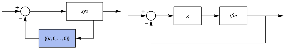
The closed-loop poles for a gain value κ:
κ = RandomReal[{0, 10}];
tfm = TransferFunctionModel[{{{k}}, (1 + s)*(2 + s)*
(3 + s)}, s];Subscript[p, cl] = TransferFunctionPoles[SystemsModelFeedbackConnect[tfm /. k -> κ]][[1, 1]]The controllable canonical state-space realization of the system:
ssm = StateSpaceModel[tfm, StateSpaceRealization -> "ControllableCompanion"]For this realization, the state feedback gains are of the form {{κ,0,…,0}}:
Chop[StateFeedbackGains[ssm, Subscript[p, cl]]] == {{κ, 0, 0}}The closed-loop poles for a gain value κ:
κ = RandomReal[{0, 10}];
tfm = TransferFunctionModel[{{{k}}, (1 + s)*(2 + s)*
(3 + s)}, s];Subscript[p, cl] = TransferFunctionPoles[SystemsModelFeedbackConnect[tfm /. k -> κ]][[1, 1]]The controllable canonical state-space realization of the system:
ssm = StateSpaceModel[tfm, StateSpaceRealization -> "ControllableCompanion"]For this realization, the state feedback gains are of the form {{κ,0,…,0}}:
Chop[StateFeedbackGains[ssm, Subscript[p, cl]]] == {{κ, 0, 0}}The state feedback and estimator gains are duals of each other:
{ssm = StateSpaceModel[{{{0, 1, 0, 0}, {0, 0, -1, 0}, {0, 0, 0, 1}, {0, 0, 11, 0}}, {{0}, {1}, {0}, {1}},
  {{1, 2, 3, 4}}, {{0}}}, SamplingPeriod -> None, SystemsModelLabels -> None], dualssm = DualSystemsModel[ssm]}
The state feedback gains of the system for a set of poles:
p = {-1, -2, -1 + I, -1 - I};
κ = StateFeedbackGains[ssm, p]
The estimator gains of the dual system for the conjugate set of poles:
ℓ = EstimatorGains[dualssm, p]The state feedback gain matrix is the conjugate transpose of the estimator gain matrix and conversely:
{κ == ℓ, ℓ == κ}State feedback does not alter the input-blocking properties of a system:
ssm = StateSpaceModel[{{{0, 1, 0}, {0, 0, 1}, {-1, -2, -2}}, {{0}, {0}, {1}}, {{4, 0, 1}}, {{0}}},
SamplingPeriod -> None, SystemsModelLabels -> None];TransferFunctionZeros[TransferFunctionModel[ssm]]The closed-loop system for a specific set of poles:
csys = StateFeedbackGains[ssm, {-3 + 2 I, -3 - 2 I, -7}, "ClosedLoopSystem"]Both the open- and closed-loop systems block the input Sin[2t]:
or = Table[OutputResponse[sys, Sin[2t], t], {sys, {ssm, csys}}];
{Plot[or[[1]], {t, 0, 15}, IconizedObject[«plotOpts»]], Plot[or[[2]], {t, 0, 3}, IconizedObject[«plotOpts»]]}
The closed-loop system becomes unobservable if the state feedback makes a pole and a zero coincident:
ssm = StateSpaceModel[{{{0, 1}, {-12, -8.}}, {{0}, {1}}, {{4, 1}}, {{0}}}, SamplingPeriod -> None,
SystemsModelLabels -> None];z = TransferFunctionZeros[TransferFunctionModel[ssm]]//FlattenThe closed-loop system with the pole coinciding with the zero:
p = {z[[1]], -8};
csys = StateFeedbackGains[ssm, p, "ClosedLoopSystem"]
The coincident pole-zero pair makes the closed-loop system unobservable:
ObservableModelQ[csys]Possible Issues (5)
The gains cannot be calculated for an uncontrollable system:
ssm = StateSpaceModel[{{{-1, 0}, {0, -3}}, {{1}, {0}}, {{1, 2}}, {{0}}}, SamplingPeriod -> None,
 SystemsModelLabels -> None];
ControllableModelQ[ssm]StateFeedbackGains[ssm, {-4, -5}]An uncontrollable descriptor system:
dssm = StateSpaceModel[{{{-5, 0}, {0, 1}}, {{0}, {0}}, {{1, 0}}, {{0}}, {{1, 0}, {0, 0}}},
 SamplingPeriod -> None, SystemsModelLabels -> None];
{ControllableModelQ[dssm], ControllableModelQ[{dssm, "Slow"}]}
The dimension of the slow subsystem:
dim = Total[Diagonal[Normal[dssm][[5]]]]None of the poles are changed:
StateFeedbackGains[dssm, RandomReal[{-8, -6}, dim], {"OpenLoopPoles", "ClosedLoopPoles"}]The gains cannot be calculated for an unstabilizable system:
StateFeedbackGains[StateSpaceModel[{{{-3, 0}, {0, 2}}, {{1}, {0}}}, SamplingPeriod -> None, SystemsModelLabels -> None], RandomInteger[{-10, -1}, 2]]The KNVD method does not handle exact systems with fewer inputs than states:
ssm = StateSpaceModel[{{{-1, 0, 1}, {-3, 1, 2}, {1, -1, 2}}, {{1, 0}, {0, 1}, {1, -2}}},
SamplingPeriod -> None, SystemsModelLabels -> None];p = {-5 + I, -5 - I, -6};
κ = StateFeedbackGains[ssm, p, Method -> "KNVD"]
StateFeedbackGains[ssm//N, p, Method -> "KNVD"]StateFeedbackGains[ssm, p, Method -> "Ackermann"]The KNVD method can give different sets of gains on different computer systems:
ssm = StateSpaceModel[{{{0, 2, 0, 0, -2, 0}, {1, 0, 0, 0, 0, -1}, {0, 1, 0, 0, 0, 0}, {0, 0, 0, 3, 0, 0},
   {2, 0, 0, 1, 0, 0}, {0, 0, -1, 0, 1, 0}}, {{1, 2}, {0, 0}, {0, 1}, {0, -1}, {0, 1}, {0, 0}}},
 SamplingPeriod -> None, SystemsModelLabels -> None];
p = {-1, -2, -3, -4, -5, -7};{$SystemID, Subscript[κ, 1] = StateFeedbackGains[ssm//N, p, Method -> "KNVD"]}{$SystemID, Subscript[κ, 2] = StateFeedbackGains[ssm//N, p, Method -> "KNVD"]}The closed-loop eigenvalues are the same:
{$SystemID, With[{ssN = Normal[ssm]}, Eigenvalues[ssN[[1]] - ssN[[2]].Subscript[κ, 1]]]}{$SystemID, With[{ssN = Normal[ssm]}, Eigenvalues[ssN[[1]] - ssN[[2]].Subscript[κ, 2]]]}Text
Wolfram Research (2010), StateFeedbackGains, Wolfram Language function, https://reference.wolfram.com/language/ref/StateFeedbackGains.html (updated 2021).
CMS
Wolfram Language. 2010. "StateFeedbackGains." Wolfram Language & System Documentation Center. Wolfram Research. Last Modified 2021. https://reference.wolfram.com/language/ref/StateFeedbackGains.html.
APA
Wolfram Language. (2010). StateFeedbackGains. Wolfram Language & System Documentation Center. Retrieved from https://reference.wolfram.com/language/ref/StateFeedbackGains.html