MassTransportPDEComponent
MassTransportPDEComponent[vars,pars]
yields a mass transport PDE term with variables vars and parameters pars.
Details
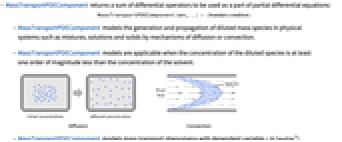
- MassTransportPDEComponent returns a sum of differential operators to be used as a part of partial differential equations:
- MassTransportPDEComponent models the generation and propagation of diluted mass species in physical systems such as mixtures, solutions and solids by mechanisms of diffusion or convection.
- MassTransportPDEComponent models are applicable when the concentration of the diluted species is at least one order of magnitude less than the concentration of the solvent.
- MassTransportPDEComponent models mass transport phenomena with dependent variable
 in [
in [![TemplateBox[{InterpretationBox[, 1], {"mol", , "/", , {"m", ^, 3}}, moles per meter cubed, {{(, "Moles", )}, /, {(, {"Meters", ^, 3}, )}}}, QuantityTF] TemplateBox[{InterpretationBox[, 1], {"mol", , "/", , {"m", ^, 3}}, moles per meter cubed, {{(, "Moles", )}, /, {(, {"Meters", ^, 3}, )}}}, QuantityTF]](Files/MassTransportPDEComponent.en/4.png) ], independent variables
], independent variables  in [
in [![TemplateBox[{InterpretationBox[, 1], "m", meters, "Meters"}, QuantityTF] TemplateBox[{InterpretationBox[, 1], "m", meters, "Meters"}, QuantityTF]](Files/MassTransportPDEComponent.en/6.png) ] and time variable
] and time variable  in [
in [![TemplateBox[{InterpretationBox[, 1], "s", seconds, "Seconds"}, QuantityTF] TemplateBox[{InterpretationBox[, 1], "s", seconds, "Seconds"}, QuantityTF]](Files/MassTransportPDEComponent.en/8.png) ].
]. - Stationary variables vars are vars={c[x1,…,xn],{x1,…,xn}}.
- Time-dependent variables vars are vars={c[t,x1,…,xn],t,{x1,…,xn}}.
- MassTransportPDEComponent provides both a conservative model to be used with compressible fluids and a non-conservative model to be used with incompressible fluids.
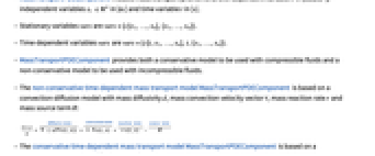
- The non-conservative time-dependent mass transport model MassTransportPDEComponent is based on a convection-diffusion model with mass diffusivity
 , mass convection velocity vector
  , mass reaction rate
  and mass source term
  :
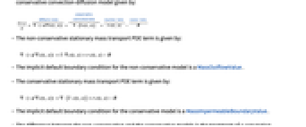
: - The conservative time-dependent mass transport model MassTransportPDEComponent is based on a conservative convection-diffusion model given by:
- The non-conservative stationary mass transport PDE term is given by:
- The implicit default boundary condition for the non-conservative model is a MassOutflowValue.
- The conservative stationary mass transport PDE term is given by:
- The implicit default boundary condition for the conservative model is a MassImpermeableBoundaryValue.
- The difference between the non-conservative and the conservative models is the treatment of a convection velocity
 .
. - The non-conservative model is the default model. The conservative model should be used when the divergence of convection velocity
 is nonzero.
 - The units of the mass transport PDE terms are in [
![TemplateBox[{InterpretationBox[, 1], {"mol", , "/(", , {"m", ^, 3}, , "s", , ")"}, moles per meter cubed second, {{(, "Moles", )}, /, {(, {{"Meters", ^, 3}, , "Seconds"}, )}}}, QuantityTF] TemplateBox[{InterpretationBox[, 1], {"mol", , "/(", , {"m", ^, 3}, , "s", , ")"}, moles per meter cubed second, {{(, "Moles", )}, /, {(, {{"Meters", ^, 3}, , "Seconds"}, )}}}, QuantityTF]](Files/MassTransportPDEComponent.en/19.png) ].
]. - The following model parameters pars can be given:
-
parameter default symbol "MassConvectionVelocity" 
 , flow velocity [
![TemplateBox[{InterpretationBox[, 1], {"m", , "/", , "s"}, meters per second, {{(, "Meters", )}, /, {(, "Seconds", )}}}, QuantityTF] TemplateBox[{InterpretationBox[, 1], {"m", , "/", , "s"}, meters per second, {{(, "Meters", )}, /, {(, "Seconds", )}}}, QuantityTF]](Files/MassTransportPDEComponent.en/22.png) ]
]"DiffusionCoefficient" IdentityMatrix  , mass diffusivity [
![TemplateBox[{InterpretationBox[, 1], {{"m", ^, 2}, , "/", , "s"}, meters squared per second, {{(, {"Meters", ^, 2}, )}, /, {(, "Seconds", )}}}, QuantityTF] TemplateBox[{InterpretationBox[, 1], {{"m", ^, 2}, , "/", , "s"}, meters squared per second, {{(, {"Meters", ^, 2}, )}, /, {(, "Seconds", )}}}, QuantityTF]](Files/MassTransportPDEComponent.en/24.png) ]
]"MassReactionRate" 0  , mass reaction rate in [1/
![TemplateBox[{InterpretationBox[, 1], "s", seconds, "Seconds"}, QuantityTF] TemplateBox[{InterpretationBox[, 1], "s", seconds, "Seconds"}, QuantityTF]](Files/MassTransportPDEComponent.en/26.png) ]
]"MassSource" 0  , mass source [
![TemplateBox[{InterpretationBox[, 1], {"mol", , "/(", , {"m", ^, 3}, , "s", , ")"}, moles per meter cubed second, {{(, "Moles", )}, /, {(, {{"Meters", ^, 3}, , "Seconds"}, )}}}, QuantityTF] TemplateBox[{InterpretationBox[, 1], {"mol", , "/(", , {"m", ^, 3}, , "s", , ")"}, moles per meter cubed second, {{(, "Moles", )}, /, {(, {{"Meters", ^, 3}, , "Seconds"}, )}}}, QuantityTF]](Files/MassTransportPDEComponent.en/28.png) ]
]"ModelForm" "NonConservative" 
"RegionSymmetry" None 
- All parameters may depend on any of
 ,
,  and
and  , as well as other dependent variables.
 - The number of independent variables
 determines the dimensions of
  and the length of
  .
. - The mass convection velocity specifies the velocity
 with which a fluid transports mass.
 - A mass reaction term
 models mass chemical reactions of masses.
 - A mass source
 models mass that is generated (positive) or absorbed (negative).
 - Possible choices for the parameter "ModelForm" are "Conservative" and "NonConservative".
- A possible choice for the parameter "RegionSymmetry" is "Axisymmetric".
- "Axisymmetric" region symmetry represents a truncated cylindrical coordinate system where the cylindrical coordinates are reduced by removing the angle variable as follows:
-
dimension reduction non-conservative equation 1D 

2D 

-
dimension reduction conservative equation 1D 

2D 

- The input specification for the parameters is exactly the same as for their corresponding operator terms.
- Coupled equations can be generated with the same input specification as with the corresponding operator terms.
- If no parameters are specified, the default mass transport PDE is:
- If the MassTransportPDEComponent depends on parameters
 that are specified in the association pars as …,keypi…,pivi,…], the parameters
  are replaced with
  .
.

Examples
open allclose allBasic Examples (3)
Define a time-dependent mass transport model:
Set up a time-dependent mass transport model with particular material parameters:
Model a 1D chemical species field in an incompressible fluid whose right side and left side are subjected to a mass concentration and inflow condition, respectively:
Set up the stationary mass transport model variables vars:
Specify the mass transport model parameters species diffusivity ![]() and fluid flow velocity
and fluid flow velocity ![]() :
:
Specify a species flux boundary condition:
Scope (23)
Basic Usage (9)
Set up a time-dependent mass transport model with numeric material parameters:
Define a 2D stationary mass transport model:
Set up a 2D stationary mass transport model with an orthotropic mass diffusion:
Set up a 2D stationary mass transport model with a diffusivity matrix:
Set up a 2D stationary mass transport model with an anisotropic diffusivity matrix:
Define a 2D stationary mass transport model with a material change:
Define a 2D stationary mass transport model with a material change and an anisotropic material:
Set up a coupled 2D stationary mass transport model:
Set up a coupled 2D transient mass transport model with cross-coupled nonlinear reaction terms:
1D (1)
Model a 1D chemical species field in an incompressible fluid whose right side and left side are subjected to a mass concentration and inflow condition, respectively:
Set up the stationary mass transport model variables vars:
Specify the mass transport model parameters species diffusivity ![]() and fluid flow velocity
and fluid flow velocity ![]() :
:
Specify a species flux boundary condition:
1D Axisymmetric (3)
2D (2)
Model mass transport of a pollutant in a 2D rectangular region in an isotropic homogeneous medium. Initially, the pollutant concentration is zero throughout the region of interest. A concentration of 3000 ![]() is maintained at a strip with dimension 0.2
is maintained at a strip with dimension 0.2 ![]() located at the center of the left boundary, while the right boundary is subject to a parallel species flow with a constant concentration of 1500
located at the center of the left boundary, while the right boundary is subject to a parallel species flow with a constant concentration of 1500 ![]() , allowing for mass transfer. A pollutant outflow of 100
, allowing for mass transfer. A pollutant outflow of 100 ![]() is applied at both the top and bottom boundaries. A diffusion coefficient of 0.833
is applied at both the top and bottom boundaries. A diffusion coefficient of 0.833 ![]() is distributed uniformly with a uniform horizontal velocity of 0.01
is distributed uniformly with a uniform horizontal velocity of 0.01 ![]() :
:
Set up the mass transport model variables vars:
Set up a rectangular domain with a width of ![]() and a height of
and a height of ![]() :
:
Specify model parameters species diffusivity ![]() and fluid flow velocity
and fluid flow velocity ![]() :
:
Set up a species concentration source of 0.2 ![]() in length at the center of the left surface:
in length at the center of the left surface:
Set up a mass transfer boundary on the right surface:
Set up an outflow flux ![]() of
of ![]() on the top and bottom surfaces:
on the top and bottom surfaces:
Symmetry boundaries can be used to reduce the size of the geometry of the model. Set up a mass transport equation:
Set up and visualize a region:
Solve and visualize the equation:
Set up a region about the symmetry axis at ![]() :
:
Solve and visualize the equation with a symmetry boundary at ![]() :
:
2D Axisymmetric (2)
3D (1)
Model a non-conservative chemical species field in a unit cubic domain, with two mass conditions at two lateral surfaces and a mass inflow through a circle with radius 0.2 ![]() at the center of the top surface, as well as an orthotropic mass diffusivity
at the center of the top surface, as well as an orthotropic mass diffusivity ![]() :
:
Set up the mass transport model variables vars:
Specify a diffusivity ![]() and a flow velocity field
and a flow velocity field ![]() :
:
Specify a flux condition ![]() of
of ![]() through a regional circle on the top surface:
through a regional circle on the top surface:
Material Regions (1)
Model a 1D chemical species transport through different material with a reaction rate in one. The right side and left side are subjected to a mass concentration and inflow condition, respectively:
Set up the stationary mass transport model variables vars:
Specify the mass transport model parameters species diffusivity ![]() and a reaction rate
and a reaction rate ![]() active in the region
active in the region ![]() :
:
Specify a species flux boundary condition:
Time Dependent (1)
Model a 1D non-conservative chemical species field and a mass flux through part of the boundary with:
Set up the time-dependent mass transport model variables vars:
Specify the mass transport model parameters mass diffusivity ![]() and mass convection velocity
and mass convection velocity ![]() :
:
Set up the equation with a mass flux ![]() of
of ![]() at the left end for the first 50 seconds:
at the left end for the first 50 seconds:
Solve the PDE with an initial condition of a zero concentration:
Nonlinear Time Dependent (1)
Model a 1D non-conservative chemical species field with a nonlinear diffusivity coefficient ![]() and an outflow condition through part of the boundary, which is expressed as follows:
and an outflow condition through part of the boundary, which is expressed as follows:
Set up the mass transport model variables vars:
Specify the nonlinear species diffusivity ![]() and fluid flow velocity
and fluid flow velocity ![]() :
:
Specify an outflow flux ![]() of
of ![]() applied at the right end:
applied at the right end:
Specify a time-dependent mass concentration surface condition:
Coupled Time Dependent (2)
Model a 1D coupled non-conservative dual chemical species field with corresponding mass flux through the left parts of the boundary:
Set up the time-dependent mass transport model variables vars for the ![]() and
and ![]() species, respectively:
species, respectively:
Specify the mass transport model parameters mass diffusivity ![]() and
and ![]() for the
for the ![]() and
and ![]() species:
species:
Set up the boundary conditions with a mass flux ![]() of 4
of 4 ![]() and 8
and 8 ![]() for
for ![]() and
and ![]() at the left end for the first 50 seconds:
at the left end for the first 50 seconds:
Model a 1D coupled chemical species field with a convection velocity and a mass flux through the left boundary:
Set up the time-dependent mass transport model variables vars for the ![]() and
and ![]() species, respectively:
species, respectively:
Specify the mass transport model parameters mass diffusivity ![]() and
and ![]() for the
for the ![]() and
and ![]() species:
species:
Set up the equation with a mass flux ![]() of 6
of 6 ![]() and 12
and 12 ![]() for
for ![]() and
and ![]() at the left end for the first 50 seconds:
at the left end for the first 50 seconds:
Applications (7)
Single Equations (4)
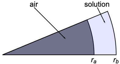
This mass transport model describes the sedimentation and diffusion of a solute under ultracentrifugation in a disk sector cell. The governing equation for describing this phenomenon is called the Lamm equation, which can be modeled with a 1D axisymmetric conservative mass transport equation:
Set up the mass transport model variable vars:
Set up a line region ![]() where
where ![]() denotes the radial position of the air-solution meniscus, which is formed during the centrifugation process, and
denotes the radial position of the air-solution meniscus, which is formed during the centrifugation process, and ![]() the radial position of the cell bottom:
the radial position of the cell bottom:
Specify the model parameter's species diffusivity ![]() in
in ![]() and fluid flow velocity
and fluid flow velocity ![]() , where
, where ![]() is the sedimentation coefficient in seconds (
is the sedimentation coefficient in seconds (![]() ) and
) and ![]() the angular velocity in
the angular velocity in ![]() :
:
Set up the parameters with an initial unity concentration:
Set up the initial conditions:
The flux is zero at both boundaries of the domain, so the boundary condition used is the MassImpermeableBoundaryValue that is applied at ![]() .This specific boundary is the implicit default boundary condition for the conservative model.
.This specific boundary is the implicit default boundary condition for the conservative model.
Visualize the concentrations at various points in time:
Model mass transport of a pollutant in a 2D rectangular region in an isotropic homogeneous medium. Initially, the pollutant concentration is zero throughout the region of interest. A concentration of 3000 ![]() is maintained at a strip with dimension 0.2
is maintained at a strip with dimension 0.2 ![]() located at the center of the left boundary, while a pollutant outflow of 100
located at the center of the left boundary, while a pollutant outflow of 100 ![]() is applied at both the top and bottom boundaries. A diffusion coefficient of 0.833
is applied at both the top and bottom boundaries. A diffusion coefficient of 0.833 ![]() is distributed uniformly, but both horizontal and vertical velocity are spatial dependent:
is distributed uniformly, but both horizontal and vertical velocity are spatial dependent:
Set up the mass transport model variables vars:
Set up a rectangular domain with a width of ![]() and a height of
and a height of ![]() :
:
Specify the model parameters species diffusivity ![]() and fluid flow velocity
and fluid flow velocity ![]() :
:
Set up a species concentration source of 0.2 ![]() length at the center of the left surface:
length at the center of the left surface:
Set up an outflow flux ![]() of
of ![]() on the top and bottom surfaces:
on the top and bottom surfaces:
Set up a Fokker–Planck equation:
Set up the mass transport model variables vars:
Specify the model parameters species diffusivity ![]() , the convection velocity term and parameters:
, the convection velocity term and parameters:
In this case, a first-order mesh is sufficient to solve the Fokker–Planck equation. Using a higher mesh order will result in an increased memory consumption. While solving, NDSolve will warn about the convection-dominant nature of the PDE:
Visualize the expected solution at the point {0,0}:
The Smoluchowski diffusion equation is a special case of the Fokker–Plank equation. Both equations can be modeled with a conservative mass transport equation:
Set up the mass transport model variables vars:
Set up a line domain with a width of 8 units:
Specify the model parameters species diffusivity ![]() and a migration term that depends on a linear potential U(x) that relates to F(x) with F(x)=-∇xU(x):
and a migration term that depends on a linear potential U(x) that relates to F(x) with F(x)=-∇xU(x):
Set up the known analytical solution:
Set up the initial conditions at ![]() from the analytical solution:
from the analytical solution:
Coupled Equations (3)
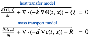
Solve a coupled heat and mass transport model:
Set up the heat transfer mass transport model variables vars:
Specify heat transfer and mass transport model parameters, heat source ![]() , thermal conductivity
, thermal conductivity ![]() , mass diffusivity
, mass diffusivity ![]() and mass source
and mass source ![]() :
:
Set up the model and initial conditions:
Solve a coupled heat transfer and mass transport model with a thermal transfer value and a mass flux value on the boundary:
Set up the heat transfer mass transport model variables vars:
Specify heat transfer and mass transport model parameters, heat source ![]() , thermal conductivity
, thermal conductivity ![]() , mass diffusivity
, mass diffusivity ![]() and mass source
and mass source ![]() :
:
Specify boundary condition parameters for a thermal convection value with an external flow temperature ![]() of 1000 K and a heat transfer coefficient
of 1000 K and a heat transfer coefficient ![]() of
of ![]() :
:
A numeric cyclic voltammetry can be performed by solving a coupled reaction model:
The underlying reaction model is given by
Set up the mass transport model variables vars:
Specify the electrochemical rate constants:
Specify mass transport model parameters, mass diffusivity ![]() and
and ![]() . The concentration of
. The concentration of ![]() at the far end is set to the bulk concentration and the concentration of
at the far end is set to the bulk concentration and the concentration of ![]() is set to 0:
is set to 0:
Set up initial conditions such that only ![]() is in bulk solution:
is in bulk solution:
Visualize the concentrations at various points in time:
Visualize the cyclic voltammogram at various points in time:
Properties & Relations (1)
Model a 1D chemical species field once with a conservative model and once with a non-conservative model. For a constant velocity flow field, both models return the same result. The right side and left side are subjected to a mass concentration and inflow conditions, respectively:
Set up the stationary mass transport model variables vars:
Specify the mass transport model parameters species diffusivity ![]() and fluid flow velocity
and fluid flow velocity ![]() :
:
Specify mass concentration boundary condition:
Possible Issues (2)
The implicit default boundary condition changes depending on the model form. For a conservative model, an implicit Neumann 0 boundary condition is equivalent to specifying an impermeable boundary condition. For a non-conservative model, an implicit Neumann 0 boundary condition is equivalent to specifying an outflow boundary condition.
Considering this, for a constant velocity field, both the conservative and non-conservative models return the same result. A comparison between the conservative and non-conservative fields are conducted based on the following models:
Set up the mass transport model variables vars:
Specify the model parameters species diffusivity ![]() and fluid flow velocity
and fluid flow velocity ![]() :
:
Set up a species concentration source of 0.2 ![]() length at the center of the left surface:
length at the center of the left surface:
Set up an outflow flux ![]() of
of ![]() on the top and bottom surfaces:
on the top and bottom surfaces:
Since the default boundary condition for a conservative model is an impermeable boundary, an impermeable boundary condition is added to the non-conservative mode:
Visualize the difference in the solutions:
The scale of the differences in the solutions is expected and comes from numerical differences in how the operators are computed.
When a discretized region is given and the mesh does not meet the quality criteria for a large convection-to-diffusion ratio, a message is generated. Model a 1D non-conservative chemical species field with a high convection velocity to diffusivity ratio, expressed as follows:
Set up the mass transport model variables vars:
Specify a nonlinear species diffusivity ![]() and fluid flow velocity
and fluid flow velocity ![]() :
:
Specify an outflow flux ![]() of
of ![]() applied at the right end:
applied at the right end:
Specify mass concentration surface conditions:
Text
Wolfram Research (2020), MassTransportPDEComponent, Wolfram Language function, https://reference.wolfram.com/language/ref/MassTransportPDEComponent.html (updated 2021).
CMS
Wolfram Language. 2020. "MassTransportPDEComponent." Wolfram Language & System Documentation Center. Wolfram Research. Last Modified 2021. https://reference.wolfram.com/language/ref/MassTransportPDEComponent.html.
APA
Wolfram Language. (2020). MassTransportPDEComponent. Wolfram Language & System Documentation Center. Retrieved from https://reference.wolfram.com/language/ref/MassTransportPDEComponent.html
