



MassTransportPDEComponent
MassTransportPDEComponent[vars,pars]
生成具有变量 vars 和参数 pars 的传质 PDE 项.
更多信息
- MassTransportPDEComponent 返回微分算子的总和,以用作偏微分方程的一部分:
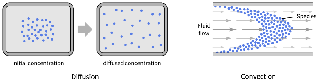
- MassTransportPDEComponent 模拟在物理系统(例如混合物、溶液和固体)中,稀释的质量物种通过扩散或对流机制的生成和传播.
- 当稀释物质的浓度比溶剂的浓度小至少一个数量级时,MassTransportPDEComponent 模型适用.
- MassTransportPDEComponent 模拟传质现象,因变量
 单位为 [
 ],自变量
 单位为 [
 ],时间变量
 单位为 [
 ].
- 平稳变量 vars 为 vars={c[x1,…,xn],{x1,…,xn}}.
- 与时间相关的变量 vars 为 vars={c[t,x1,…,xn],t,{x1,…,xn}}.
- MassTransportPDEComponent 既提供了用于可压缩流体的保守模型,也提供了用于不可压缩流体的非保守模型.
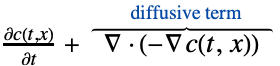
- 非保守时变传质模型 MassTransportPDEComponent 基于对流扩散模型,其中质量扩散率为
 ,质量对流速度矢量为
 ,质量反应速率为
 ,质量源项为
 :
- 保守时变传质模型 MassTransportPDEComponent 基于保守的对流扩散模型,由下式给出:
- 非保守平稳传质 PDE 项由下式给出:
- 非保守模型的隐式默认边界条件是 MassOutflowValue.
- 保守平稳传质 PDE 项由下式给出:
- 保守模型的隐式默认边界条件是 MassImpermeableBoundaryValue.
- 非保守模型与保守模型的区别在于对对流速度
 的处理.
- 非保守模型是默认模型. 当对流速度
 的散度不为零时,应使用保守模型.
- 传质 PDE 项的单位是
 ].
- 可以给出以下模型参数 pars:
-
参数 缺省值 符号 "MassConvectionVelocity" 
 ,流速,单位为 [
 ]
"DiffusionCoefficient" IdentityMatrix  ,质量扩散率,单位为 [
 ]
"MassReactionRate" 0  ,质量反应率,单位为 [
 ]
"MassSource" 0  ,质量源,单位为 [
 ]
"ModelForm" "NonConservative" 
"RegionSymmetry" None 
- 所有参数可能取决于
 、
 和
 中的任何一个,以及其他因变量.
- 自变量
 的数量确定
 的维数和
 的长度.
- 质量对流速度指定了流体传输质量的速度
 .
- 质量反应项
 模拟质量的质量化学反应.
- 质量源
 模拟产生(正)或吸收(负)的质量.
- 参数 "ModelForm" 的可能选项是 "Conservative" 或 "NonConservative".
- 参数 "RegionSymmetry" 的可用选择是 "Axisymmetric".
- "Axisymmetric" 区域对称性表示截断圆柱坐标系,其中通过移除角度变量来减少圆柱坐标,如下所示:
-
维度 缩减 非保守方程 1D 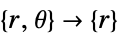

2D 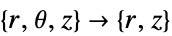

-
维度 缩减 保守方程 1D 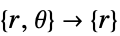

2D 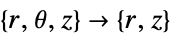

- 参数的输入规范与其对应的运算符项完全相同.
- 耦合方程可以使用与相应的运算符相同的输入规范来生成.
- 如果未指定任何参数,则默认的传质 PDE 为:
- 如果 MassTransportPDEComponent 取决于在关联 pars 中指定为 …,keypi…,pivi,… 的参数
 ,则参数
 用
 替换.





范例
打开所有单元 关闭所有单元基本范例 (3)
MassTransportPDEComponent[{c[t, x], t, {x}}, <||>]MassTransportPDEComponent[{c[t, x], t, {x}}, <|"DiffusionCoefficient" -> d|>]对不可压缩流体中的一维化学物种场建模,该流体的右侧和左侧分别受到质量浓度和流入条件的影响:

vars = {c[x], {x}};
Ω = Line[{{0}, {1}}];

pars = <|"DiffusionCoefficient" -> 0.026, "MassConvectionVelocity" -> {0.1}|>;Subscript[Γ, flux] = MassFluxValue[x == 0, vars, pars, <|"MassFlux" -> 1|>]Subscript[Γ, C] = MassConcentrationCondition[x == 1, vars, pars, <|"MassConcentration" -> 0|>]eqn = MassTransportPDEComponent[vars, pars] == Subscript[Γ, flux]cfun = NDSolveValue[{eqn, Subscript[Γ, C]}, c, x∈Ω];Plot[cfun[x], x∈Ω, Rule[...]]范围 (23)
基本用法 (9)
MassTransportPDEComponent[{c[t, x], t, {x}}, <|"DiffusionCoefficient" -> 2|>]MassTransportPDEComponent[{c[x, y], {x, y}}, <|"DiffusionCoefficient" -> 1.2 * 10 ^ -6|>]MassTransportPDEComponent[{c[x, y], {x, y}}, <|"DiffusionCoefficient" -> {1, 2}|>]MassTransportPDEComponent[{c[x, y], {x, y}}, <|"DiffusionCoefficient" -> IdentityMatrix[2]|>]MassTransportPDEComponent[{c[x, y], {x, y}}, <|"DiffusionCoefficient" -> {{2, 3}, {0, 4}}|>]MassTransportPDEComponent[{c[x, y], {x, y}}, <|"DiffusionCoefficient" -> If[x < 1 / 2, 1, 2] * IdentityMatrix[2]|>]MassTransportPDEComponent[{c[x, y], {x, y}}, <|"DiffusionCoefficient" -> If[x < 1 / 2, {{1, 0}, {0, 1}}, {{2, 1}, {0, 3}}]|>]MassTransportPDEComponent[{{c1[x, y], c2[x, y]}, {x, y}}, <|"DiffusionCoefficient" -> {{1, 10 ^ -3}, {2 * 10 ^ -3, 1}}|>]MassTransportPDEComponent[{{c1[t, x, y], c2[t, x, y]}, t, {x, y}}, <|"DiffusionCoefficient" -> {{1, 10 ^ -3}, {2 * 10 ^ -3, 1}}, "MassReactionRate" -> {{c1[t, x, y] * c2[t, x, y], c1[t, x, y]}, {0, Sqrt[c1[t, x, y]]}}|>]一维 (1)
对不可压缩流体中的一维化学物种场建模,该流体的右侧和左侧分别受到质量浓度和流入条件的影响:

vars = {c[x], {x}};
Ω = Line[{{0}, {1}}];

pars = <|"DiffusionCoefficient" -> 0.026, "MassConvectionVelocity" -> {0.1}|>;Subscript[Γ, flux] = MassFluxValue[x == 0, vars, pars, <|"MassFlux" -> 1|>]Subscript[Γ, C] = MassConcentrationCondition[x == 1, vars, pars, <|"MassConcentration" -> 0|>]eqn = MassTransportPDEComponent[vars, pars] == Subscript[Γ, flux]cfun = NDSolveValue[{eqn, Subscript[Γ, C]}, c, x∈Ω];Plot[cfun[x], x∈Ω, Rule[...]]1D 轴对称 (3)
MassTransportPDEComponent[{c[r], {r}}, <|"DiffusionCoefficient" -> {{d}}, "MassConvectionVelocity" -> {Subscript[v, r]}, "RegionSymmetry" -> "Axisymmetric"|>]MassTransportPDEComponent[{c[r], {r}}, <|"DiffusionCoefficient" -> {{d}}, "MassConvectionVelocity" -> {Subscript[v, r]}, "RegionSymmetry" -> "Axisymmetric", "ModelForm" -> "Conservative"|>]lammEquation = MassTransportPDEComponent[{c[t, r], t, {r}}, <|"DiffusionCoefficient" -> {{d}}, "RegionSymmetry" -> "Axisymmetric", "MassConvectionVelocity" -> {sc ω ^ 2 r}, "ModelForm" -> "Conservative"|>] == 0Simplify[Activate[lammEquation]]二维 (2)
模拟污染物在各向同性均质介质中二维矩形区域的质量传输. 最初,整个目标区域的污染物浓度为零. 在左边界中心处尺寸为 0.2  的条带上保持 3000
 的浓度,而右边界经受浓度为 1500
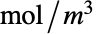 的平行物质流动,允许传质. 在顶部和底部边界都有 100
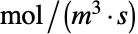 的污染物流出. 0.833
 的扩散系数以 0.01
 的均匀水平速度均匀分布:

vars = {c[x, y], {x, y}};

Ω = Rectangle[{0, 0}, {20, 10}];

pars = <|"DiffusionCoefficient" -> 0.833, "MassConvectionVelocity" -> {0.01, 0}|>;
Subscript[Γ, concentration] = MassConcentrationCondition[x == 0 && y ≤ 5.1 && y ≥ 4.9, vars, pars, <|"MassConcentration" -> 3000|>]Subscript[Γ, transfer] = MassTransferValue[x == 20, vars, pars, <|"AmbientConcentration" -> 1500, "MassTransferCoefficient" -> 5|>]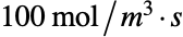

Subscript[Γ, flux] = MassFluxValue[y == 0 || y == 10, vars, pars, <|"MassFlux" -> -100|>]eqn = MassTransportPDEComponent[vars, pars] == Subscript[Γ, transfer] + Subscript[Γ, flux]cfun = NDSolveValue[{eqn, Subscript[Γ, concentration]}, c, {x, y}∈Ω];ContourPlot[cfun[x, y], {x, y}∈Ω, ...]vars = {c[x, y], {x, y}};
pars = <|"DiffusionCoefficient" -> 1, "MassSource" -> 1|>;Ω = RegionDifference[Rectangle[{-1, 0}, {1, 1}], Rectangle[{-1 / 2, 0}, {1 / 2, 1 / 2}]];
RegionPlot[Ω, AspectRatio -> Automatic]cfun = NDSolveValue[{MassTransportPDEComponent[vars, pars] == 0, MassConcentrationCondition[y == 0, vars, pars, <|"MassConcentration" -> 0|>]}, c[x, y], {x, y}∈Ω];
ContourPlot[cfun, {x, y}∈Ω]
Ω = RegionDifference[Rectangle[{0, 0}, {1, 1}], Rectangle[{0, 0}, {1 / 2, 1 / 2}]];
Show[Graphics[{{Dashed, Thick, Gray, Line[{{0, -0.1}, {0, 1.1}}]}}], RegionPlot[Ω, AspectRatio -> Automatic]]
cfun = NDSolveValue[{MassTransportPDEComponent[vars, pars] == MassSymmetryValue[x == 0, vars, pars], MassConcentrationCondition[y == 0, vars, pars, <|"MassConcentration" -> 0|>]}, c[x, y], {x, y}∈Ω];
ContourPlot[cfun, {x, y}∈Ω]
2D 轴对称 (2)
MassTransportPDEComponent[{c[r, z], {r, z}}, <|"DiffusionCoefficient" -> d * IdentityMatrix[2], "MassConvectionVelocity" -> {Subscript[v, r], Subscript[v, z]}, "RegionSymmetry" -> "Axisymmetric"|>]MassTransportPDEComponent[{c[r, z], {r, z}}, <|"DiffusionCoefficient" -> d * IdentityMatrix[2], "MassConvectionVelocity" -> {Subscript[v, r], Subscript[v, z]}, "RegionSymmetry" -> "Axisymmetric", "ModelForm" -> "Conservative"|>]三维 (1)
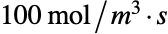
对单位立方域中的非保守化学物种场进行建模,其中在两个侧面有两个质量条件,并且在顶面中心半径为 0.2  的圆上有质量流入,以及正交各向异性质量扩散率为
 :

vars = {c[x, y, z], {x, y, z}};
Ω = Cuboid[{0, 0, 0}, {1, 1, 1}];

pars = <|"DiffusionCoefficient" -> {{1, 0, 0}, {0, 5, 0}, {0, 0, 10}}, "MassConvectionVelocity" -> {0, 10, 0}|>;Subscript[Γ, CC] = {MassConcentrationCondition[x == 0, vars, <|"MassConcentration" -> 0|>], MassConcentrationCondition[x == 1, vars, <|"MassConcentration" -> 1|>]}
Subscript[Γ, flux] = MassFluxValue[z == 1 && (x - 0.5) ^ 2 + (y - 0.5) ^ 2 ≤ 0.04, vars, pars, <|"MassFlux" -> 100|>]eqn = MassTransportPDEComponent[vars, pars] == Subscript[Γ, flux]cfun = NDSolveValue[{eqn, Subscript[Γ, CC]}, c, {x, y, z}∈Ω];GraphicsRow[Table[SliceContourPlot3D[cfun[x, y, z], sl, {x, y, z}∈Ω, ...], {...}]]材料区域 (1)
给定化学物种在一种材料内的反应速率,模拟一维化学物种穿过不同材料的过程. 右侧和左侧分别受到质量浓度和流入条件的影响:

vars = {c[x], {x}};
Ω = Line[{{0}, {1}}];


pars = <|"DiffusionCoefficient" -> 0.01, "MassReactionRate" -> If[x > 1 / 2, 1, 0]|>;Subscript[Γ, flux] = MassFluxValue[x == 0, vars, pars, <|"MassFlux" -> 1|>]Subscript[Γ, C] = MassConcentrationCondition[x == 1, vars, pars, <|"MassConcentration" -> 0|>]eqn = MassTransportPDEComponent[vars, pars] == Subscript[Γ, flux]cfun = NDSolveValue[{eqn, Subscript[Γ, C]}, c, x∈Ω];Show[Plot[cfun[x], x∈Ω, Rule[...]], Graphics[...]]随时间变化 (1)
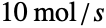
用以下内容对一维非守恒化学物种场和穿过部分边界的质量通量建模:

vars = {c[t, x], t, {x}};
Ω = Line[{{0}, {1}}];

pars = <|"DiffusionCoefficient" -> 0.01, "MassConvectionVelocity" -> {0.02}|>;
model = MassTransportPDEComponent[vars, pars] == MassFluxValue[x == 0, vars, pars, <|"MassFlux" -> Piecewise[{{10, t ≤ 50}, {0, t > 50}}]|>]cfun = NDSolveValue[{model, c[0, x] == 0}, c, {t, 0, 100}, x∈Ω];Manipulate[Show[Plot[cfun[t, x], ...], Graphics[...]], {{t, 30}, 0, 100, 2.5}, Rule[...]]非线性时间相关 (1)
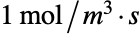
对一维非保守化学物种场进行建模,其中非线性扩散系数为  ,并具有通过部分边界的流出条件,其表示如下:

vars = {c[t, x], t, {x}};
Ω = Line[{{0}, {1}}];

pars = <|"DiffusionCoefficient" -> {{0.001 * Log[c[t, x] ^ 2 + 1]}}, "MassConvectionVelocity" -> {0.02}|>;
Subscript[Γ, flux] = MassFluxValue[x == 1, vars, pars, <|"MassFlux" -> -1|>]Subscript[Γ, C] = MassConcentrationCondition[x == 0, vars, pars, <|"MassConcentration" -> 100 + 0.1 * t|>]ics = c[0, x] == 100;eqn = MassTransportPDEComponent[vars, pars] == Subscript[Γ, flux]cfun = NDSolveValue[{eqn, ics, Subscript[Γ, C]}, c, {t, 0, 500}, x∈Ω];Manipulate[Show[Plot[cfun[t, x], ...], Graphics[...]], {{t, 30}, 0, 500, 1}, Rule[...]]耦合时间相关 (2)
对给出了边界的左侧部分相应的质量通量的一维耦合非守恒二重化学物种场建模:


vars = {{Subscript[c, 1][t, x], Subscript[c, 2][t, x]}, t, {x}};
Ω = Line[{{0}, {1}}];


pars = <|"DiffusionCoefficient" -> {{0.01, 0}, {0, 0.02}}|>;设置边界条件,在最初的50秒内,  和
 在左端的质量通量
 分别为 4
 和 8
 :
Subscript[Γ, flux] = MassFluxValue[x == 0, vars, pars, <|"MassFlux" -> {If[t ≤ 50, 4, 0], If[t ≤ 50, 8, 0]}|>]eqn = MassTransportPDEComponent[vars, pars] == Subscript[Γ, flux]ics = {Subscript[c, 1][0, x] == 0, Subscript[c, 2][0, x] == 0};{c1fun, c2fun} = NDSolveValue[{eqn, ics}, {Subscript[c, 1], Subscript[c, 2]}, {t, 0, 100}, {x}∈Ω];Manipulate[Show[Plot[{c1fun[t, x], c2fun[t, x]}, ..., PlotLegends -> {"SubscriptBox[c, 1](x)", "SubscriptBox[c, 2](x)"}], Graphics[...]], {{t, 30}, 0, 100, 2.5}, Rule[...]]对给出了对流速度和穿过左边界的质量通量的一维耦合化学物种场建模:


vars = {{Subscript[c, 1][t, x], Subscript[c, 2][t, x]}, t, {x}};
Ω = Line[{{0}, {1}}];


pars = <|"DiffusionCoefficient" -> {{0.02, 0}, {0, 0.02}}, "MassConvectionVelocity" -> {{{0.02}, {0}}, {{0}, {0.02}}}|>;设置方程,在最初的50秒内,  和
 在左端的质量通量
 分别为 6
 和 12
 :
Subscript[Γ, flux] = MassFluxValue[x == 0, vars, pars, <|"MassFlux" -> {{Piecewise[{{6, t ≤ 50}, {0, t > 50}}], 0}, {0, Piecewise[{{12, t ≤ 50}, {0, t > 50}}]}}|>];eqn = MassTransportPDEComponent[vars, pars] == Subscript[Γ, flux]ics = {Subscript[c, 1][0, x] == 0, Subscript[c, 2][0, x] == 0};{c1fun, c2fun} = NDSolveValue[{eqn, ics}, {Subscript[c, 1], Subscript[c, 2]}, {t, 0, 100}, {x}∈Ω];Manipulate[Show[Plot[{c1fun[t, x], c2fun[t, x]}, ..., PlotLegends -> {"SubscriptBox[c, 1](x)", "SubscriptBox[c, 2](x)"}], Graphics[...]], {{t, 30}, 0, 100, 2.5}, Rule[...]]应用 (7)
单一方程 (4)
该传质模型描述了在圆盘扇形单元中超速离心情况下溶质的沉降和扩散. 描述这种现象的控制方程称为 Lamm 方程,可用一维轴对称保守传质方程建模:
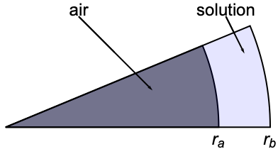
vars = {c[t, r], t, {r}};设置一个线区域  ,其中
 表示在离心过程中形成的空气溶液弯液面的径向位置,
 表示单元底部的径向位置:
Subscript[r, a] = 5.8;
Subscript[r, b] = 7.2;
Ω = Line[{{Subscript[r, a]}, {Subscript[r, b]}}];
指定模型参数的物种扩散率  ,单位为
 ,以及流体的流速
 ,其中
 是沉降系数,单位为秒 (
 ),
 是角速度,单位为
 :
pars = <|"DiffusionCoefficient" -> {d}, "RegionSymmetry" -> "Axisymmetric", "MassConvectionVelocity" -> {sc ω ^ 2 r}, "ModelForm" -> "Conservative"|>;parameters = {c0 -> 1, sc -> 1.562*^-12, ω -> 5236, d -> 1.279*^-7};pde = {MassTransportPDEComponent[vars, pars] == 0, ic} /. parameters;在区域的两个边界处通量为零,因此使用的边界条件为 MassImpermeableBoundaryValue,被应用于 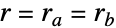 处. 该特定边界是保守模型的隐式默认边界条件.
pde = {MassTransportPDEComponent[vars, pars] == 0, ic} /. parameters;Cfun = NDSolveValue[pde, c, {t, 0, 2525}, r∈ NDSolve`FEM`ToGradedMesh[Ω, <|"Alignment" -> "Right", "ElementCount" -> 700|>]]Plot[{Cfun[0, r], Cfun[101, r], Cfun[404, r], Cfun[1010, r], Cfun[2525, r]}, {r, Subscript[r, a], Subscript[r, b]}, PlotRange -> {0, 1.5}, AxesLabel -> {r, "C"}, PlotLegends -> {"t=0 s", "t=101 s", "t=404 s", "t=1010 s", "t=2525 s"}]模拟污染物在各向同性均质介质中二维矩形区域的质量传输. 最初,整个目标区域的污染物浓度为零. 在左边界中心处尺寸为 0.2  的条带上保持 3000
 的浓度,在顶部和底部边界都有 100
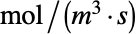 的污染物流出. 扩散系数为 0.833
 ,呈均匀分布,但水平和垂直速度均与空间有关:

vars = {c[x, y], {x, y}};

Ω = Rectangle[{0, 0}, {20, 10}];

pars = <|"DiffusionCoefficient" -> 0.833, "MassConvectionVelocity" -> {0.01x ^ 2, -0.02y}|>;
Subscript[Γ, C] = MassConcentrationCondition[x == 0 && 4.9 ≤ y ≤ 5.1, vars, pars, <|"MassConcentration" -> 3000|>]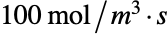

Subscript[Γ, flux] = MassFluxValue[y == 0 || y == 10, vars, pars, <|"MassFlux" -> -10|>]eqn = {MassTransportPDEComponent[vars, pars] == Subscript[Γ, flux], Subscript[Γ, C]}cfun = NDSolveValue[eqn, c, {x, y}∈Ω];ContourPlot[cfun[x, y], {x, y}∈Ω, Rule[...]]
vars = {c[t, x, y], t, {x, y}};Ω = Rectangle[{-10, -10}, {10, 10}];
pars = <|"ModelForm" -> "Conservative", "DiffusionCoefficient" -> {{0, 0}, {0, d}}, "MassConvectionVelocity" -> {y, -2ξ ω y - x}, d -> 1 / 10, ω -> 1, ξ -> 1 / 20, μ -> {5, 5}, σ -> 1 / 9 * IdentityMatrix[2]|>;ics = c[0, x, y] == PDF[MultinormalDistribution[μ, σ] /. pars, {x, y}]eqn = {MassTransportPDEComponent[vars, pars] == 0, ics}在这种情况下,一阶网格足以求解 Fokker–Planck 方程. 使用更高阶数的网格将导致内存消耗增加. 求解时,NDSolve 将警告 PDE 的对流主导性质:
cfun = Monitor[NDSolveValue[eqn, c, {t, 0, 100}, {x, y}∈Ω, Method -> {"PDEDiscretization" -> {"MethodOfLines", {"SpatialDiscretization" -> {"FiniteElement", "MeshOptions" -> {"MaxCellMeasure" -> 0.05, "MeshOrder" -> 1}}}}}, EvaluationMonitor :> (monitor = Row[{"t = ", CForm[t]}])], monitor]
Plot[cfun[t, 0, 0], {t, 0, 100}, Ticks -> {Automatic, Range[0, 0.18, 0.02]}, GridLines -> {Automatic, Range[0, 0.18, 0.02]}]Smoluchowski 扩散方程是 Fokker–Plank 方程的特例. 这两个方程都可以用一个保守的质量传输方程建模:

vars = {c[t, x], t, {x}};Ω = Line[{{-8}, {8}}];指定模型参数物种扩散率  和依赖于线性势 U(x) 的迁移项,与 F(x) 的关系为 F(x)=-∇xU(x):
U[x_] := γ * x
pars = <|"ModelForm" -> "Conservative", "DiffusionCoefficient" -> {{d}}, "MassConvectionVelocity" -> β * (-Grad[U[x], {x}]), d -> 1, γ -> 1, β -> 1|>;solution[t_, x_] := Evaluate[With[{x0 = 0, t0 = 0},
1 / Sqrt[4 π d (t - t0)] * Exp[-(x - x0 + d β γ (t - t0)) ^ 2 / (4d * (t - t0))]] /. pars]
ics = c[1 / 10, x] == solution[1 / 10, x];eqn = {MassTransportPDEComponent[vars, pars] == 0, ics}cfun = NDSolveValue[eqn, c, {t, 1 / 10, 1}, {x}∈Ω];frames = Table[Plot[cfun[t, x], {x}∈Ω, PlotRange -> {0, 1}], {t, 1 / 10, 1, 1 / 10}];
ListAnimate[frames, SaveDefinitions -> True]
Plot[{solution[1, x] - cfun[1, x]}, {x}∈Ω, PlotRange -> All]耦合方程 (3)

hvars = {Θ[t, x], t, {x}};
mvars = {c[t, x], t, {x}};
Ω = Line[{{0}, {1}}];指定传热和传质模型参数,热源  ,导热系数
 ,质量扩散系数
 和质量源
 :
pars = <|"ThermalConductivity" -> 0.01, "HeatSource" -> 0.2 * R, "DiffusionCoefficient" -> 0.01, "MassSource" -> R, R -> -10 ^ -3 * Θ[t, x] * c[t, x]|>;eqn = {HeatTransferPDEComponent[hvars, pars] == 0, MassTransportPDEComponent[mvars, pars] == 0}ics = {Θ[0, x] == 200 + 800x, c[0, x] == 800};{Tfun, cfun} = NDSolveValue[{eqn, ics}, {Θ, c}, {t, 0, 10}, {x}∈Ω];Manipulate[Plot[{cfun[t, x], Tfun[t, x]}, {x}∈Ω, ...], {{t, 1.3}, 0, 10}, Rule[...]]
hvars = {Θ[t, x], t, {x}};
mvars = {c[t, x], t, {x}};
Ω = Line[{{0}, {1}}];指定传热和传质模型参数,热源  ,导热系数
 ,质量扩散系数
 和质量源
 :
pars = <|"ThermalConductivity" -> 0.01, "HeatSource" -> 0.2 * R, "DiffusionCoefficient" -> 0.01, "MassSource" -> R, R -> -10 ^ -3 * Θ[t, x] * c[t, x]|>;指定热对流值的边界条件参数,其中外部流体温度  为 1000 K,传热系数
 为
 :
pars["BC1"] = <|"AmbientTemperature" -> 1000, "HeatTransferCoefficient" -> 0.1|>;eqn = {HeatTransferPDEComponent[hvars, pars] == HeatTransferValue[x == 1, hvars, pars, "BC1"], MassTransportPDEComponent[mvars, pars] == NeumannValue[20, x == 0 || x == 1]}ics = {Θ[0, x] == 200 + 800x, c[0, x] == 800};{Tfun, cfun} = NDSolveValue[{eqn, ics}, {Θ, c}, {t, 0, 10}, {x, 0, 1}];Manipulate[Plot[{cfun[t, x], Tfun[t, x]}, {x}∈Ω, ...], {{t, 1.7}, 0, 10}, Rule[...]]

vars = {{cA[t, x], cB[t, x]}, t, {x}};
Ω = Line[{{0}, {1 / 40}}];cAbulk = 1;
dA = 10 ^ -5;dB = 10 ^ -5;k0 = 10 ^ -5;α = 1 / 2;β = 1 / 2;ef0 = 0;rtbyf = 25.7 10 ^ -3;
kc[t_] := Evaluate[k0 Exp[-α / rtbyf (e[t] - ef0)]]
ka[t_] := Evaluate[k0 Exp[β / rtbyf (e[t] - ef0)]]ts = 1;ν = -1;e1 = 1 / 2;
e[t_] := Evaluate[Piecewise[{{e1 + ν t, 0 ≤ t ≤ ts}, {e1 + 2 ν ts - ν t, ts ≤ t ≤ 2 ts}}]]指定质量传输模型参数,物质扩散率  和
 . 将远端的浓度
 设置为整体浓度,将浓度
 设为 0:
pars = <|"DiffusionCoefficient" -> {{dA, 0}, {0, dB}}, "BoundaryCondition1" -> <|"AmbientConcentration" -> {ka[t] / kc[t] cB[t, x], kc[t] / ka[t] cA[t, x]}, "MassTransferCoefficient" -> {kc[t], ka[t]}|>, "BoundaryCondition2" -> <|"MassConcentration" -> {cAbulk, 0}|>|>;eqn = {MassTransportPDEComponent[vars, pars] == MassTransferValue[x == 0, vars, pars, "BoundaryCondition1"], MassConcentrationCondition[x == 1 / 40, vars, pars, "BoundaryCondition2"]};
ics = {cA[0, x] == cAbulk, cB[0, x] == 0};tmax = 2 ts;
{cAfun, cBfun} = NDSolveValue[{eqn, ics}, {cA, cB}, {t, 0, tmax}, {x}∈Ω];Manipulate[Plot[{cAfun[t, x], cBfun[t, x]}, {x, 0, 1 / 20}, ...], {...}, Rule[...]]Manipulate[ParametricPlot[{-(e[t] - ef0), kc[t] (cAfun[t, 0] - (ka[t] cBfun[t, 0]) / kc[t])}, {t, 0, tmax}, ...], {...}, Rule[...]]属性和关系 (1)
分别使用保守模型和非保守模型对一维化学物种场进行建模. 对于恒定速度的流场,两个模型返回的结果相同. 右侧和左侧分别受到质量浓度和流入条件的影响:


vars = {c[x], {x}};
Ω = Line[{{0}, {1}}];

pars1 = <|"DiffusionCoefficient" -> 0.026, "MassConvectionVelocity" -> {0.1}|>;
pars2 = Join[pars1, <|"ModelForm" -> "Conservative"|>];massConditons1 = MassConcentrationCondition[x == 1, vars, pars1, <|"MassConcentration" -> 0|>];massConditons2 = MassConcentrationCondition[x == 1, vars, pars2, <|"MassConcentration" -> 0|>];Subscript[Γ, flux1] = MassFluxValue[x == 0, vars, pars1, <|"MassFlux" -> 1|>];
Subscript[Γ, flux2] = MassFluxValue[x == 0, vars, pars2, <|"MassFlux" -> 1|>];eqn1 = MassTransportPDEComponent[vars, pars1] == Subscript[Γ, flux1];
eqn2 = MassTransportPDEComponent[vars, pars2] == Subscript[Γ, flux2];cfun1 = NDSolveValue[{eqn1, massConditons1}, c, x∈Ω]cfun2 = NDSolveValue[{eqn2, massConditons2}, c, x∈Ω]Plot[{cfun1[x] - cfun2[x]}, x∈Ω, AxesLabel -> {"x", "c"}, PlotLegends -> "Expressions"]可能存在的问题 (2)
隐含的默认边界条件随模型形式而变化. 对于守恒模型,隐式 Neumann 0 边界条件相当于指定不可渗透的边界条件. 对于非守恒模型,隐式 Neumann 0 边界条件相当于指定流出边界条件.
考虑到这一点,对于恒定速度场,守恒模型和非守恒模型返回相同的结果. 基于以下模型对守恒域和非守恒域进行比较:


vars = {c[x, y], {x, y}};Ω = Rectangle[{0, 0}, {2, 1}];

pars1 = <|"DiffusionCoefficient" -> 1, "MassConvectionVelocity" -> {0.01, -0.02}|>;
pars2 = Join[pars1, <|"ModelForm" -> "Conservative"|>];
Subscript[Γ, concentration1] = MassConcentrationCondition[x == 0 && 0.4 ≤ y ≤ 0.6, vars, pars1, <|"MassConcentration" -> 1|>]Subscript[Γ, concentration2] = MassConcentrationCondition[x == 0 && 0.4 ≤ y ≤ 0.6, vars, pars2, <|"MassConcentration" -> 1|>]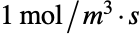

Subscript[Γ, flux1] = MassFluxValue[y == 0 || y == 10, vars, pars1, <|"MassFlux" -> -1|>]Subscript[Γ, flux2] = MassFluxValue[y == 0 || y == 10, vars, pars2, <|"MassFlux" -> -1|>]由于保守模型的默认边界条件是不可渗透边界,因此将不可渗透边界条件添加到非保守模式:
Subscript[Γ, imp] = MassImpermeableBoundaryValue[(x == 0 && (y < 4.9 || y > 5.1)) || x == 20, vars, pars1]eqn1 = {MassTransportPDEComponent[vars, pars1] == Subscript[Γ, flux1] + Subscript[Γ, imp], Subscript[Γ, concentration1]};
eqn2 = {MassTransportPDEComponent[vars, pars2] == Subscript[Γ, flux2], Subscript[Γ, concentration2]};cfun1 = NDSolveValue[eqn1, c, {x, y}∈Ω];
cfun2 = NDSolveValue[eqn2, c, {x, y}∈Ω];ContourPlot[cfun1[x, y] - cfun2[x, y], {x, y}∈Ω, PlotLegends -> Automatic]当给出离散区域并且网格不满足高对流扩散比的质量标准时,将生成一条消息. 模拟具有高对流速度与扩散比的一维非保守化学物种场,表示如下:

vars = {c[t, x], t, {x}};
Ω = Line[{{0}, {1}}];

pars = <|"DiffusionCoefficient" -> 0.005, "MassConvectionVelocity" -> {1}|>;
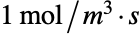
Subscript[Γ, flux] = MassFluxValue[x == 1, vars, pars, <|"MassFlux" -> -1|>]massConditons = MassConcentrationCondition[x == 0, vars, pars, <|"MassConcentration" -> 100 + 0.1 * t|>];ics = c[0, x] == 100;eqn = MassTransportPDEComponent[vars, pars] == Subscript[Γ, flux]cfun = NDSolveValue[{eqn, ics, massConditons}, c, {t, 0, 500}, x∈NDSolve`FEM`ToElementMesh[Ω]];
cfun = NDSolveValue[{eqn, ics, massConditons}, c, {t, 0, 500}, x∈NDSolve`FEM`ToElementMesh[Ω, "MaxCellMeasure" -> 0.01]]文本
Wolfram Research (2020),MassTransportPDEComponent,Wolfram 语言函数,https://reference.wolfram.com/language/ref/MassTransportPDEComponent.html (更新于 2021 年).
CMS
Wolfram 语言. 2020. "MassTransportPDEComponent." Wolfram 语言与系统参考资料中心. Wolfram Research. 最新版本 2021. https://reference.wolfram.com/language/ref/MassTransportPDEComponent.html.
APA
Wolfram 语言. (2020). MassTransportPDEComponent. Wolfram 语言与系统参考资料中心. 追溯自 https://reference.wolfram.com/language/ref/MassTransportPDEComponent.html 年