PeriodicBoundaryCondition[u[x1,…],pred,f]
represents a periodic boundary condition ![]() for all xtarget on the boundary of the region given to NDSolve where pred is True.
for all xtarget on the boundary of the region given to NDSolve where pred is True.
PeriodicBoundaryCondition[a+b u[x1,…],pred,f]
represents a generalized periodic boundary condition ![]() .
.


PeriodicBoundaryCondition
PeriodicBoundaryCondition[u[x1,…],pred,f]
represents a periodic boundary condition ![]() for all xtarget on the boundary of the region given to NDSolve where pred is True.
for all xtarget on the boundary of the region given to NDSolve where pred is True.
PeriodicBoundaryCondition[a+b u[x1,…],pred,f]
represents a generalized periodic boundary condition ![]() .
.
Details
- PeriodicBoundaryCondition is used together with differential equations to describe boundary conditions in functions such as NDSolve.
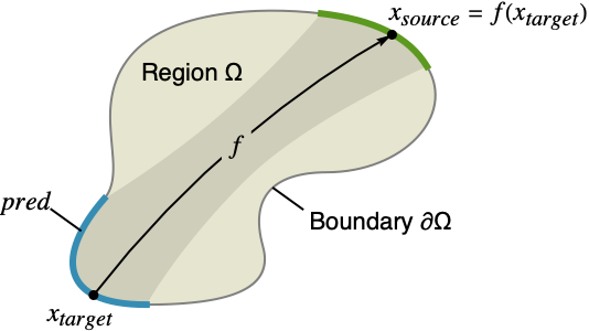
- In NDSolve[eqns,{u1,u2,…},{x1,x2,…}∈Ω], xi are the independent variables, uj are the dependent variables, and Ω is the region with boundary ∂Ω.
- Locations where periodic boundary conditions might be specified are shown in blue. They appear on the boundary ∂Ω of the region Ω and specify the relation of the solution at those locations to the locations shown in green. The function f maps from the blue locations to the green locations.
- In the special case of rectangular region Ω, a boundary equation u[…,xi,min,…]u[…,xi,max,…] is taken to be equivalent to PeriodicBoundaryCondition[u[…,xi,…],xixi,max,f] with f=TranslationTransform[{…,0,xi,min-xi,max,0,…}]. »
- Any logical combination of equalities and inequalities in the independent variables x1,… may be used for the predicate pred.
- In PeriodicBoundaryCondition[a+b u[x1,…],pred,f], for any point xtarget in the part of ∂Ω where pred is True, then xsource=f[xtarget] should be a point in ∂Ω where pred is not True.
- With PeriodicBoundaryCondition[a+b u[x1,…],pred,f], in NDSolve the system matrices are modified so that the solution values u[xtarget] approximately satisfy u[xsource]==a+b u[xtarget] for all xtarget on the boundary of Ω where pred is True.
- Boundary conditions for
 , including implicit Neumann 0 conditions, will also be mapped to
  .
. - In PeriodicBoundaryCondition[a+b u[x1,…],pred,f], both a and b are scalar values that may depend on any of the independent variables xi, including time.
- Antiperiodic boundaries may be specified using PeriodicBoundaryCondition[-u[x1,…],pred,f].
- Common values for a and b include:
-
u[x1,…] periodic boundary condition -u[x1,…] anti-periodic boundary condition a u[x1,…] scaled periodic boundary condition u[x1,…]+b offset periodic boundary condition - For finite element approximations, PeriodicBoundaryCondition operates on nodes in 1D, on edges in 2D and on faces in 3D.
Examples
open all close allBasic Examples (2)
Find 5 eigenvalues and eigenvectors of a Laplacian with periodic boundary conditions:
{vals, funs} = NDEigensystem[{-u''[x], PeriodicBoundaryCondition[u[x], x == 2π, Function[X, X - 2π]]}, u[x], {x, 0, 2π}, 5];Compare the eigenvalues with the expected analytical eigenvalues:
vals - Flatten[Join[{0}, Table[{n ^ 2, n ^ 2}, {n, 1, 2}]]]Plot[funs, {x, 0, 2π}]Inspect to see that the bounds are periodic:
(funs /. x -> 0) - (funs /. x -> 2π)Solve a Poisson equation with periodic boundary conditions on curved boundaries:
Ω = RegionDifference[RegionUnion[Disk[], Rectangle[{0, -1}, {2, 1}]], Disk[{2, 0}]];ufun = NDSolveValue[{-Subsuperscript[∇, {x, y}, 2]u[x, y] == If[(x - 1 / 4) ^ 2 + y ^ 2 ≤ 1 / 4, 1, 0], PeriodicBoundaryCondition[u[x, y], x ^ 2 + y ^ 2 == 1, Function[X, X + {2, 0}]], DirichletCondition[u[x, y] == 0, (10 ^ -14 < x < 2 && (y == -1 || y == 1))]}, u, {x, y}∈Ω];cp = ContourPlot[ufun[x, y], {x, y}∈Ω, ColorFunction -> "TemperatureMap", AspectRatio -> Automatic]Visualize the periodic solution:
Show[MapAt[Translate[#, {2, 0}]&, cp, 1], cp, MapAt[Translate[#, {-2, 0}]&, cp, 1], PlotRange -> All]Scope (15)
1D Eigenvalue Problems (7)
Find 5 eigenvalues and eigenvectors of a Mathieu equation:
{vals, funs} = NDEigensystem[{-u''[x] + 4 Cos[2x] u[x], PeriodicBoundaryCondition[u[x], x == 2π, Function[X, X - 2π]]}, u[x], {x, 0, 2π}, 5];Plot[funs, {x, 0, 2π}]Inspect to see that the bounds are periodic:
(funs /. x -> 0) - (funs /. x -> 2π){vals, funs} = NDEigensystem[{-u''[x] + 4 Cos[2x] u[x], u[0] == u[2π]}, u[x], {x, 0, 2π}, 5];
(funs /. x -> 0) - (funs /. x -> 2π)Find 5 eigenvalues and eigenvectors of a Laplacian with antiperiodic bounds:
{vals, funs} = NDEigensystem[{-u''[x], PeriodicBoundaryCondition[-u[x], x == 2π, TranslationTransform[{-2π}]]}, u[x], {x, 0, 2π}, 5];valsPlot[funs, {x, 0, 2π}]Inspect to see that the eigenvectors add up at the endpoints:
Plus[funs /. x -> 0, funs /. x -> 2π]Find 9 eigenvalues and eigenvectors of the Meissner equation on a refined mesh:
w[x_] := If[x < 0, 1, 9]
{vals, funs} = NDEigensystem[{-1 / w[x]u''[x], PeriodicBoundaryCondition[u[x], x == 1 / 2, TranslationTransform[{-1}]]}, u[x], {x, -1 / 2, 1 / 2}, 9, Method -> {
	"SpatialDiscretization" -> {"FiniteElement", {"MeshOptions" -> {MaxCellMeasure -> 0.001}}}
	}];
Compare the eigenvalues with the expected analytical eigenvalues:
α = ArcCos[-7 / 8];
vals - Join[{0}, Flatten[Table[{(2 * n * π + α) ^ 2, (2 * (n + 1) * π - α) ^ 2, (2 * (n + 1) * π) ^ 2, (2 * (n + 1) * π) ^ 2}, {n, 0, 1}]]]Plot[funs, {x, -1 / 2, 1 / 2}]Find 5 eigenvalues and eigenvectors of a Sturm–Liouville operator with a symmetric potential:
V[x_] := Cos[x];
{vals, funs} = NDEigensystem[{-u''[x] - (V''[x] - V'[x] ^ 2) u[x], PeriodicBoundaryCondition[u[x], x == 2π, TranslationTransform[{-2π}]]}, u[x], {x, 0, 2π}, 5];valsRecompute the eigenvalues with higher resolution:
{vals, funs} = NDEigensystem[{-u''[x] - (V''[x] - V'[x] ^ 2) u[x], PeriodicBoundaryCondition[u[x], x == 2π, TranslationTransform[{-2π}]]}, u[x], {x, 0, 2π}, 5, Method -> {"SpatialDiscretization" -> {"FiniteElement", "MeshOptions" -> {"MaxCellMeasure" -> 0.001}}}];valsPlot[funs, {x, 0, 2π}]Find 5 periodic eigenvalues and eigenvectors of a Sturm–Liouville operator with an unsymmetrical potential:
V[x_] := Cos[x] + x;
{vals, funs} = NDEigensystem[{-u''[x] - (V''[x] - V'[x] ^ 2) u[x], PeriodicBoundaryCondition[u[x], x == 2π, TranslationTransform[{-2π}]]}, u[x], {x, 0, 2π}, 5];valsPlot[funs, {x, 0, 2π}]Find 5 antiperiodic eigenvalues and eigenvectors of a Sturm–Liouville operator with an unsymmetrical potential:
V[x_] := Cos[x] + x;
{vals, funs} = NDEigensystem[{-u''[x] - (V''[x] - V'[x] ^ 2) u[x], PeriodicBoundaryCondition[-u[x], x == 2π, TranslationTransform[{-2π}]]}, u[x], {x, 0, 2π}, 5];valsPlot[funs, {x, 0, 2π}]Inspect to see that the eigenvectors add up at the endpoints:
Plus[funs /. x -> 0, funs /. x -> 2π]Find 5 relational antiperiodic eigenvalues and eigenvectors of a Sturm–Liouville operator with an unsymmetrical potential:
V[x_] := Cos[x] + x;
{vals, funs} = NDEigensystem[{-u''[x] - (V''[x] - V'[x] ^ 2) u[x], PeriodicBoundaryCondition[-2u[x], x == 2π, TranslationTransform[{-2π}]]}, u[x], {x, 0, 2π}, 5];valsPlot[funs, {x, 0, 2π}]Inspect to see that the eigenvectors match the relation at the endpoints:
(funs /. x -> 0) - (-2) * (funs /. x -> 2π)1D+Time PDE Problems (2)
Solve a 1D Schrödinger equation with periodic boundary conditions:
ufun = NDSolveValue[{I D[u[t, x], t] == -D[u[t, x], {x, 2}], u[0, x] == Exp[-(x ^ 2)],
	PeriodicBoundaryCondition[u[t, x], x == -5, TranslationTransform[{10}]]
}, u, {t, 0, 5}, {x}∈Line[{{-5}, {5}}]]plots = Table[Plot[Abs[ufun[t, x]], {x, -5, 5}, PlotRange -> {0, 1}], {t, 0, 3, .1}];
ListAnimate[plots]Solve a 1D wave equation with periodic boundary conditions:
f[x_] = D[0.125 Erf[(x - 0.5) / 0.125], x];
vInit[x_] = -D[f[x], x];
ufun = NDSolveValue[{D[u[t, x], {t, 2}] - D[u[t, x], {x, 2}] == NeumannValue[-Derivative[1, 0][u][t, x], x == 0 || x == 1]
	, u[0, x] == f[x]
	, Derivative[1, 0][u][0, x] == vInit[x]
	, PeriodicBoundaryCondition[u[t, x], x == 0, TranslationTransform[{1}]]
	}, u, {t, 0, 2}, {x, 0, 1}];
Visualize the periodic wavefunction:
plots = Table[Plot[ufun[t, x], {x, 0, 1}], {t, 0, 2, .1}];
ListAnimate[plots]
The previous example used ![]() as a target. In this case, the target is placed where the flux is entering the periodic domain.
as a target. In this case, the target is placed where the flux is entering the periodic domain.
If instead ![]() is the target, the wave pulse inverts when reaching
is the target, the wave pulse inverts when reaching ![]() and then moves backward. At
and then moves backward. At ![]() an implicit Neumann 0 boundary condition imposes a hard boundary condition and the pulse is reflecting off that hard boundary:
an implicit Neumann 0 boundary condition imposes a hard boundary condition and the pulse is reflecting off that hard boundary:
ufunM = NDSolveValue[{D[u[t, x], {t, 2}] - D[u[t, x], {x, 2}] == NeumannValue[-Derivative[1, 0][u][t, x], x == 0 || x == 1]
	, u[0, x] == f[x]
	, Derivative[1, 0][u][0, x] == vInit[x]
	, PeriodicBoundaryCondition[u[t, x], x == 1, TranslationTransform[{-1}]]
	}, u, {t, 0, 2}, {x, 0, 1}];
Compare the two periodic wavefunctions:
plots = Table[Plot[{ufun[t, x], ufunM[t, x]}, {x, 0, 1}, PlotRange -> 1.15, PlotLegends -> LineLegend[{"x=0", "x=1"}, LegendLabel -> "target"]],
	{t, 0, 2, .1}];
ListAnimate[plots]
2D PDE Problems (4)
Set up a rectangular region to solve a PDE with a DirichletCondition on the top and bottom:
Ω = Rectangle[{0, 0}, {2, 1}];
pde = -Subsuperscript[∇, {x, y}, 2]u[x, y] == If[1.25 ≤ x ≤ 1.75 && 0.25 ≤ y ≤ 0.5, 1., 0.];
Subscript[Γ, D] = DirichletCondition[u[x, y] == 0, (y == 0 || y == 1) && 0 < x ≤ 2];
To implement a periodic boundary condition, specify a mapping f from the target (x==0) to the source (x==2):
f = TranslationTransform[{2, 0}];Visualize the region Ω and the source of the periodic boundary condition in green and the target in blue:
Show[RegionPlot[Ω], Graphics[{Thickness[0.015], #}]& /@ {{Darker[Green], TransformedRegion[#, f]}, {Darker[Blue], #}}&[Line[{{0, 0}, {0, 1}}]], AspectRatio -> Automatic]Specify the periodic boundary condition using the mapping function f:
pbc = PeriodicBoundaryCondition[u[x, y], x == 0, f];Solve and visualize the equation:
ufun = NDSolveValue[{pde, pbc, Subscript[Γ, D]}, u, {x, y}∈Ω];
ContourPlot[ufun[x, y], {x, y}∈Ω, ColorFunction -> "TemperatureMap", AspectRatio -> Automatic]
Find the solution to a Laplace-type equation over a rectangle with a DirichletCondition at the lower-left corner and periodic boundary conditions linking the opposite sides:
ufun = NDSolveValue[{-Laplacian[u[x, y], {x, y}] == 10 x ^ 5 * y ^ 3,
DirichletCondition[u[x, y] == 0, x == 0 && y == 0], PeriodicBoundaryCondition[u[x, y], 0 ≤ y ≤ 1 && x == 1, FindGeometricTransform[{{0, 0}, {0, 1}}, {{1, 0}, {1, 1}}][[2]]], PeriodicBoundaryCondition[u[x, y], 0 ≤ x ≤ 1 && y == 1, FindGeometricTransform[{{0, 0}, {1, 0}}, {{0, 1}, {1, 1}}][[2]]]}, u, {x, y}∈Rectangle[{0, 0}, {1, 1}]];Plot3D[ufun[x, y], {x, y}∈Rectangle[{0, 0}, {1, 1}]]Inspect the difference of the solution at the boundaries:
GraphicsColumn[{Plot[ufun[x, 0] - ufun[x, 1], {x, 0, 1}], Plot[ufun[0, y] - ufun[1, y], {y, 0, 1}]}]Note that the DirichletCondition in the lower-left corner has been propagated to the remaining corners:
{ufun[0, 0], ufun[1, 0], ufun[0, 1], ufun[1, 1]}Ω = ImplicitRegion[1 ≤ x ^ 2 + y ^ 2 ≤ 4 && x - y ≥ 0 && x ≥ 0 && y ≥ 0, {x, y}];Show the region and the boundaries:
Show[RegionPlot[Ω], ContourPlot[{-y == 0, 1 - x ^ 2 - y ^ 2 == 0, -4 + x ^ 2 + y ^ 2 == 0, -x + y == 0}, {x, 1 / Sqrt[2] - .1, 2 + .1}, {y, -.1, Sqrt[2] + .1}, ContourStyle -> {Darker[Green], Orange, Orange, Darker[Blue]}], AspectRatio -> Automatic, PlotRange -> {{0.6, 2.1}, {-0.1, 1.5}}]Find a mapping f that maps from the target (blue) to the source (green):
{error, f} = FindGeometricTransform[{{1, 0}, {2, 0}}, {{1 / Sqrt[2], 1 / Sqrt[2]}, {Sqrt[2], Sqrt[2]}}];Solve a Poisson equation with internal heat generation and a fixed temperature set on the orange boundaries, and a periodic boundary condition linking the green source and the blue target boundary:
ufun = NDSolveValue[{-Subsuperscript[∇, {x, y}, 2]u[x, y] == If[1.4 ≤ x ≤ 1.6 && 0 ≤ y ≤ 0.1, 1., 0.], PeriodicBoundaryCondition[u[x, y], (y - x) == 0, f], DirichletCondition[u[x, y] == 0, (x ^ 2 + y ^ 2 == 1 || x ^ 2 + y ^ 2 == 4) && !(y - x) > -10 ^ -7]}, u, {x, y}∈Ω];Inspect to see that the periodic boundaries have the same values:
Plot[{ufun[x, 0] - ufun@@InverseFunction[f][{x, 0}]}, {x, 1, 2}, PlotRange -> All]ContourPlot[ufun[x, y], {x, y}∈Ω, ColorFunction -> "TemperatureMap", Contours -> 21]Compare to an antiperiodic solution:
ufun = NDSolveValue[{-Subsuperscript[∇, {x, y}, 2]u[x, y] == If[1.4 ≤ x ≤ 1.6 && 0 ≤ y ≤ 0.1, 1., 0.], PeriodicBoundaryCondition[-u[x, y], (y - x) == 0, f], DirichletCondition[u[x, y] == 0, (x ^ 2 + y ^ 2 == 1 || x ^ 2 + y ^ 2 == 4) && !(y - x) > -10 ^ -7]}, u, {x, y}∈Ω];
ContourPlot[ufun[x, y], {x, y}∈Ω, ColorFunction -> "TemperatureMap", Contours -> 21]Ω = Rectangle[{0, 0}, {2, 1}];
pde = -Subsuperscript[∇, {x, y}, 2]u[x, y] == If[1.25 ≤ x ≤ 1.75 && 0.25 ≤ y ≤ 0.5, 1., 0.];The lower and upper parts are subject to a DirichletCondition:
Subscript[Γ, D] = DirichletCondition[u[x, y] == 0, (y == 0 || y == 1) && 0 < x ≤ 2];The left-hand edge is the target of the relational boundary condition of the right-hand edge (the source):
a = -1 / 20;b = 2;
pbc = PeriodicBoundaryCondition[a + b * u[x, y], x == 0 && 0 ≤ y ≤ 1, TranslationTransform[{2, 0}]];Solve and visualize the equation:
ufun = NDSolveValue[{pde, pbc, Subscript[Γ, D]}, u, {x, y}∈Ω];
ContourPlot[ufun[x, y], {x, y}∈Ω, ColorFunction -> "TemperatureMap", AspectRatio -> Automatic]Inspect to see that the periodic boundaries have the correct relation:
Plot[{a + b * ufun[0, y] - ufun[2, y]}, {y, 0, 1}, PlotRange -> All]2D+Time PDE Problems (1)
Solve a 2D time-dependent Schrödinger equation with a potential fitting the box and with periodic boundary conditions:
ufun = NDSolveValue[{I D[u[t, x, y], t] == -D[u[t, x, y], {x, 2}] - D[u[t, x, y], {y, 2}] - 20 Cos[Pi x / 10] Cos[Pi y / 10] u[t, x, y], u[0, x, y] == Exp[-((x - 1) ^ 2 + y ^ 2)] Exp[I y], PeriodicBoundaryCondition[u[t, x, y], x == -5, TranslationTransform[{10, 0}]],
PeriodicBoundaryCondition[u[t, x, y], y == -5, TranslationTransform[{0, 10}]]}, u, {t, 0, 3}, {x, y}∈Rectangle[{-5, -5}, {5, 5}]];plots = Table[Plot3D[Abs[ufun[t, x, y]], {x, -5, 5}, {y, -5, 5}, PlotRange -> {0, 1}], {t, 0, 3, .1}];
ListAnimate[plots]3D Problems (1)
Solve a Poisson equation in a cuboid with periodic boundary conditions:
Ω = Cuboid[{0, 0, 0}, {5, 1, 1}];ufun = NDSolveValue[{-Laplacian[u[x, y, z], {x, y, z}] == 1, DirichletCondition[u[x, y, z] == 0, 0 < x < 5], PeriodicBoundaryCondition[u[x, y, z], x == 0, TranslationTransform[{5, 0, 0}]]}, u, {x, y, z}∈Ω]SliceContourPlot3D[ufun[x, y, z], {{"XStackedPlanes", {0, 1.5, 3.5, 5}}, {"YStackedPlanes", 1}, {"ZStackedPlanes", 1}}, {x, y, z}∈Ω, ColorFunction -> "TemperatureMap", Boxed -> False, Axes -> False]Applications (1)
Compute eigenvalues of a Laplacian in polar coordinates over a Disk:
pvals = NDEigenvalues[{-Laplacian[u[r, ϕ], {r, ϕ}, "Polar"], DirichletCondition[u[r, ϕ] == 0, r == 1 && 0 < ϕ ≤ 2π], PeriodicBoundaryCondition[u[r, ϕ], ϕ == 0, TranslationTransform[{0, 2 π}]]}, u[r, ϕ], {r, 0, 1}, {ϕ, 0, 2π}, 3]Analytically compute the eigenvalues of a Laplacian in Cartesian coordinates over a Disk:
avals = DEigenvalues[{-Laplacian[u[x, y], {x, y}], DirichletCondition[u[x, y] == 0, True]}, u[x, y], {x, y}∈Disk[], 3]Compare the eigenvalues computed:
pvals - avalsNumerically compute the eigenvalues of a Laplacian in Cartesian coordinates over a Disk:
cvals = NDEigenvalues[{-Laplacian[u[x, y], {x, y}], DirichletCondition[u[x, y] == 0, True]}, u[x, y], {x, y}∈Disk[], 3]Compare the numerically computed eigenvalues computed in Cartesian coordinates with the analytical solution:
cvals - avalsCompare the numerically computed eigenvalues:
cvals - pvalsPossible Issues (8)
Exclusively specifying periodic boundary condition for stationary PDEs may result in a non-unique solution. In some cases, the system may not be solvable at all:
V[x_] := Cos[x];
ufun = NDSolveValue[{u''[x] + (V''[x] - V'[x] ^ 2) u[x] == -1,
PeriodicBoundaryCondition[u[x], x == 2π, TranslationTransform[{-2 π}]]}, u, {x, 0, 2π}]Plot[ufun[x], {x, 0, 2π}]Specify a DirichletCondition on the source boundary:
V[x_] := Cos[x];
ufun = NDSolveValue[{u''[x] + (V''[x] - V'[x] ^ 2) u[x] == -1,
DirichletCondition[u[x] == 0, x == 0],
PeriodicBoundaryCondition[u[x], x == 2π, TranslationTransform[{-2 π}]]}, u, {x, 0, 2π}]Plot[ufun[x], {x, 0, 2π}]The source for the mapping f of the PeriodicBoundaryCondition need not necessarily be on the boundary of a domain:
domain = {x, 0, 2π};
f1 = TranslationTransform[{-π}];V[x_] := Cos[x];
ufun = NDSolveValue[{u''[x] + (V''[x] - V'[x] ^ 2) u[x] == -1,
DirichletCondition[u[x] == 0, x == 0],
PeriodicBoundaryCondition[u[x], x == 2π, f1]}, u, domain]Plot[ufun[x], {x, 0, 2π}]ufun[f1[{2π}]] - ufun[2π]Compare to the solution where the source is on the boundary:
f2 = TranslationTransform[{-2π}];V[x_] := Cos[x];
ufun = NDSolveValue[{u''[x] + (V''[x] - V'[x] ^ 2) u[x] == -1,
DirichletCondition[u[x] == 0, x == 0],
PeriodicBoundaryCondition[u[x], x == 2π, f2]}, u, {x, 0, 2π}]Plot[ufun[x], {x, 0, 2π}]DirichletCondition cannot be present on the target boundary:
V[x_] := Cos[x];
ufun = NDSolveValue[{u''[x] + (V''[x] - V'[x] ^ 2) u[x] == -1,
DirichletCondition[u[x] == 0, x == 2π],
PeriodicBoundaryCondition[u[x], x == 2π, TranslationTransform[{-2 π}]]}, u, {x, 0, 2π}]Moving the DirichletCondition to the source boundary works:
V[x_] := Cos[x];
ufun = NDSolveValue[{u''[x] + (V''[x] - V'[x] ^ 2) u[x] == -1,
DirichletCondition[u[x] == 0, x == 0],
PeriodicBoundaryCondition[u[x], x == 2π, TranslationTransform[{-2 π}]]}, u, {x, 0, 2π}, Method -> "FiniteElement"]Periodic boundary conditions propagate the solution of a PDE from the source to the target boundary. The choice of which boundary is considered source and which is target has an influence on the solution of the PDE.
Consider a rectangular domain and an asymmetric Poisson equation:
Ω = Rectangle[{0, 0}, {2, 1}];
pde = -Subsuperscript[∇, {x, y}, 2]u[x, y] == If[1.25 ≤ x ≤ 1.75 && 0.25 ≤ y ≤ 0.5, 1., 0.];
The lower and upper parts are subject to a DirichletCondition:
Subscript[Γ, D] = DirichletCondition[u[x, y] == 0, (y == 0 || y == 1) && 0 < x ≤ 2];First, the left-hand edge is the target boundary to the right-hand edge (the source):
pbc = PeriodicBoundaryCondition[u[x, y], x == 0 && 0 ≤ y ≤ 1, TranslationTransform[{2, 0}]];Solve and visualize the equation:
ufun = NDSolveValue[{pde, pbc, Subscript[Γ, D]}, u, {x, y}∈Ω];
ContourPlot[ufun[x, y], {x, y}∈Ω, ColorFunction -> "TemperatureMap", AspectRatio -> Automatic]
Inspect the values at the periodic boundaries:
Plot[{ufun[0, y] - ufun[2, y]}, {y, 0, 1}, PlotRange -> All]In the second example, the right-hand edge is a target boundary to the left-hand edge (the source):
Subscript[Γ, D] = DirichletCondition[u[x, y] == 0, (y == 0 || y == 1) && 0 ≤ x < 2];
pbc = PeriodicBoundaryCondition[u[x, y], x == 2 && 0 ≤ y ≤ 1, TranslationTransform[{-2, 0}]];Solve and visualize the equation:
ufun = NDSolveValue[{pde, pbc, Subscript[Γ, D]}, u, {x, y}∈Ω];
ContourPlot[ufun[x, y], {x, y}∈Ω, ColorFunction -> "TemperatureMap", AspectRatio -> Automatic]
Inspect the values at the periodic boundaries:
Plot[{ufun[0, y] - ufun[2, y]}, {y, 0, 1}, PlotRange -> All]Periodic boundary conditions propagate the solution of a PDE from a source region to the target region. The direction of the mapping has an influence on the solution of the PDE.
Consider a rectangular domain and an asymmetric Poisson equation:
Ω = Rectangle[{0, 0}, {2, 1}];
pde = -Subsuperscript[∇, {x, y}, 2]u[x, y] == If[1.5 ≤ x ≤ 2 && 0 ≤ y ≤ 0.25, 1., 0.];The lower and upper parts are subject to a DirichletCondition:
Subscript[Γ, D] = DirichletCondition[u[x, y] == 0, (y == 0 || y == 1) && 0 < x ≤ 2];Map the lower right to the higher left-hand side and the higher right to the lower left-hand side:
mapping = FindGeometricTransform[{{2, 1}, {2, 0}}, {{0, 0}, {0, 1}}][[2]];The left-hand side is a target boundary to the right-hand side:
pbc = PeriodicBoundaryCondition[u[x, y], x == 0 && 0 ≤ y ≤ 1, mapping];Solve and visualize the equation:
ufun = NDSolveValue[{pde, pbc, Subscript[Γ, D]}, u, {x, y}∈Ω];
ContourPlot[ufun[x, y], {x, y}∈Ω, ColorFunction -> "TemperatureMap", AspectRatio -> Automatic]Compare to mapping in the same direction but with flipped edges; the lower right to the lower left-hand side and the higher right to the higher left-hand side:
mapping = FindGeometricTransform[{{2, 0}, {2, 1}}, {{0, 0}, {0, 1}}][[2]];The left-hand side is a target boundary to the right-hand side:
pbc = PeriodicBoundaryCondition[u[x, y], x == 0 && 0 ≤ y ≤ 1, mapping];Solve and visualize the equation:
ufun = NDSolveValue[{pde, pbc, Subscript[Γ, D]}, u, {x, y}∈Ω];
ContourPlot[ufun[x, y], {x, y}∈Ω, ColorFunction -> "TemperatureMap", AspectRatio -> Automatic]Periodic boundary conditions relate the solution of a PDE from the source to the target boundary. Boundary conditions present, also implicit ones, at the source will affect the solution at the target.
To exemplify the behavior, consider a time-dependent equation discretized with the finite element method. An initial condition u, implicit Neumann zero boundary conditions on both sides and no PeriodicBoundaryCondition are specified:
ufun = NDSolveValue[{D[u[t, x], t] - D[u[t, x], {x, 2}] == 0, u[0, x] == Sin[x]}, u, {t, 0, 1}, {x, -π, π}, Method -> {"MethodOfLines", "SpatialDiscretization" -> {"FiniteElement"}}]Visualize the solution at various times:
frames = Table[Plot[ufun[t, x], {x, -π, π}, PlotRange -> {-1, 1}], {t, 0, 1, 0.1}];
ListAnimate[frames, SaveDefinitions -> True]
Note that at both spatial boundaries the implicit Neumann 0 boundary conditions are satisfied.
When a PeriodicBoundaryCondition is used on a source boundary that has an implicit Neumann 0 boundary condition, then that condition will be mapped to the target boundary.
Following is the solution of the same equation and initial condition as previously and an additional periodic boundary condition that has its source on the left and its target on the right:
ufun = NDSolveValue[{D[u[t, x], t] - D[u[t, x], {x, 2}] == 0, u[0, x] == Sin[x], PeriodicBoundaryCondition[u[t, x], x == π, Function[X, X - 2π]]}, u, {t, 0, 1}, {x, -π, π}, Method -> {"MethodOfLines", "SpatialDiscretization" -> {"FiniteElement"}}]Visualize the solution at various times:
frames = Table[Plot[ufun[t, x], {x, -π, π}, PlotRange -> {-1, 1}], {t, 0, 1, 0.1}];
ListAnimate[frames, SaveDefinitions -> True]
Note how the solution value at the implicit Neumann 0 boundary condition on the left is mapped to the right.
This is the expected behavior for the finite element method. The tensor product grid method behaves differently, as that method does not have implicit boundary conditions:
ufunTPG = NDSolveValue[{D[u[t, x], t] - D[u[t, x], {x, 2}] == 0, u[0, x] == Sin[x], u[t, -π] == u[t, π]}, u, {t, 0, 1}, {x, -π, π}, Method -> {"MethodOfLines", "SpatialDiscretization" -> {"TensorProductGrid"}}]Visualize the tensor product grid solution at various times:
frames = Table[Plot[ufunTPG[t, x], {x, -π, π}, PlotRange -> {-1, 1}], {t, 0, 1, 0.1}];
ListAnimate[frames, SaveDefinitions -> True]
A similar behavior can be achieved with the finite element method by specifying a DirichletCondition on the left and a PeriodicBoundaryCondition:
ufunFEM = NDSolveValue[{D[u[t, x], t] - D[u[t, x], {x, 2}] == 0, u[0, x] == Sin[x], PeriodicBoundaryCondition[u[t, x], x == π, Function[X, X - 2π]], DirichletCondition[u[t, x] == Sin[-π], x == -π]}, u, {t, 0, 1}, {x, -π, π}, Method -> {"MethodOfLines", "SpatialDiscretization" -> {"FiniteElement"}}]Visualize the difference between the finite element and tensor product grid solutions at various times:
frames = Table[Plot[ufunFEM[t, x] - ufunTPG[t, x], {x, -π, π}, PlotRange -> {-5 10 ^ -4, 5 10 ^ -4}], {t, 0, 1, 0.1}];
ListAnimate[frames, SaveDefinitions -> True]
Alternatively, a DirichletCondition could be specified at each side.
Periodic boundary conditions relate the solution of a PDE from the source to the target boundary. Boundary conditions present, including implicit ones, at the source will affect the solution at the target. Multiple periodic boundary conditions can be used to enforce continuous derivatives.
Set up a region and a helper function that takes periodic boundary conditions as arguments:
Ω = Rectangle[{0, 0}, {2, 1}];
fun[pbcs__] := NDSolveValue[{-Laplacian[u[x, y], {x, y}] == If[(1.25 ≤ x + 2 ≤ 1.75 || 1.25 ≤ x ≤ 1.75) && 0.25 ≤ y ≤ 0.5, 1., 0.],
	pbcs,
	DirichletCondition[u[x, y] == 0, (y == 0 || y == 1) && 0 < x < 2]}, u, {x, y}∈Ω, Method -> {"FiniteElement", "MeshOptions" -> {"MaxCellMeasure" -> 0.0001, "MeshElementType" -> TriangleElement}}];
Set up plotting options and a helper function to create periodic plots:
opts = {PlotRange -> All, AspectRatio -> Automatic, ColorFunction -> "TemperatureMap", Frame -> {True, True}, PlotRangePadding -> None, ImageSize -> Large};
periodicPlot[cp_] := Show[MapAt[Translate[#, {2, 0}]&, cp, 1], cp, MapAt[Translate[#, {-2, 0}]&, cp, 1], PlotRange -> All]
Solve the PDE with a single periodic boundary condition on the left-hand side:
ufun = fun[PeriodicBoundaryCondition[u[x, y], x == 0 && 0 ≤ y ≤ 1, TranslationTransform[{2, 0}]]];Visualize a periodic contour plot of the solution:
periodicPlot[ContourPlot[ufun[x, y], {x, y}∈Ω, Evaluate[opts]]]Visualize a periodic stream density plot of the gradient of the solution:
periodicPlot[StreamDensityPlot[Evaluate@{-Grad[ufun[x, y], {x, y}], ufun[x, y]}, {x, y}∈Ω, StreamScale -> Tiny, Evaluate[opts]]]Note that the gradient is not continuous. This because of the implicit Neumann value that is present at the source location.
Similarly, visualize a periodic density plot of the norm of the gradient of the solution:
periodicPlot[DensityPlot[Evaluate[Norm@Grad[ufun[x, y], {x, y}]], {x, y}∈Ω, Evaluate[opts]]]Specifying a second periodic boundary condition enforces a continuous derivative. Solve the PDE with periodic boundary conditions on both the left- and right-hand sides:
ufun = fun[PeriodicBoundaryCondition[u[x, y], x == 0 && 0 ≤ y ≤ 1, TranslationTransform[{2, 0}]], PeriodicBoundaryCondition[u[x, y], x == 2 && 0 ≤ y ≤ 1, TranslationTransform[{-2, 0}]]];Visualize a periodic contour plot of the solution. As expected, the solution changes, since the implicit Neumann value is now eliminated:
periodicPlot[ContourPlot[ufun[x, y], {x, y}∈Ω, Evaluate[opts]]]Visualize a periodic stream density plot of the gradient of the solution. Note that now the gradient is continuous:
periodicPlot[StreamDensityPlot[Evaluate@{-Grad[ufun[x, y], {x, y}], ufun[x, y]}, {x, y}∈Ω, StreamScale -> Tiny, Evaluate[opts]]]Similarly, visualize a periodic density plot of the norm of the gradient of the solution and find that the norm of the gradient is also continuous:
periodicPlot[DensityPlot[Evaluate[Norm@Grad[ufun[x, y], {x, y}]], {x, y}∈Ω, Evaluate[opts]]]This approach works on unstructured meshes.
Periodic boundary conditions, like Neumann values, operate on edges in 2D and surfaces in 3D. This means that sufficient nodes need to be present in a finite element mesh to make periodic boundary conditions work.
Generate a finite element mesh and visualize the mesh nodes:
mesh = NDSolve`FEM`ToElementMesh["Coordinates" -> {{0., 0.}, {0.25, 0.}, {0.5, 0.}, {0.75, 0.}, {1., 0.}, {0., 0.5}, {0.25, 0.5}, {0.5, 0.5}, {0.75, 0.5}, {1., 0.5}, {0., 1.}, {0.25, 1.}, {0.5, 1.}, {0.75, 1.}, {1., 1.}}, "MeshElements" -> {NDSolve`FEM`QuadElement[{{1, 2, 7, 6}, {2, 3, 8, 7}, {3, 4, 9, 8}, {4, 5, 10, 9}, {6, 7, 12, 11}, {7, 8, 13, 12}, {8, 9, 14, 13}, {9, 10, 15, 14}}]}];
Show[
	mesh["Wireframe"],
	mesh["Wireframe"["MeshElement" -> "PointElements", "MeshElementIDStyle" -> LightDarkSwitched[Black, White]]]]
Solve a PDE with a periodic boundary condition that maps a single point:
pde = Laplacian[u[x, y], {x, y}] == 0;
bc = DirichletCondition[u[x, y] == (x - 1 / 2) ^ 2, Or[x == 1, x < 0.5]];
NDSolveValue[{pde, bc
	, PeriodicBoundaryCondition[u[x, y], 0.5 < x < 1, Function[X, X - {1, 0}]]
	}, u, Element[{x, y}, mesh]]
To fix this, specify a predicate for the periodic boundary condition that covers an edge:
NDSolveValue[{pde, bc
	, PeriodicBoundaryCondition[u[x, y], 0.5 ≤ x < 1, Function[X, X - {1, 0}]]
	}, u, Element[{x, y}, mesh]]
Neat Examples (1)
Specify a region to solve a wave equation over a box:
Ω = RegionUnion[Rectangle[{0, 0}, {4, 1}], Rectangle[{1, -1}, {2, 0}], Rectangle[{1, 1}, {2, 2}]];Set up the mapping functions so that the colored edges match. The dashed lines are the respective targets:
f1 = FindGeometricTransform[{{1, 0}, {0, 0}}, {{1, 0}, {1, -1}}][[2]];
f2 = FindGeometricTransform[{{1, -1}, {2, -1}}, {{4, 0}, {3, 0}}][[2]];
f3 = FindGeometricTransform[{{2, 0}, {2, -1}}, {{2, 0}, {3, 0}}][[2]];
f4 = FindGeometricTransform[{{0, 0}, {0, 1}}, {{4, 0}, {4, 1}}][[2]];
f5 = FindGeometricTransform[{{1, 2}, {2, 2}}, {{4, 1}, {3, 1}}][[2]];
f6 = FindGeometricTransform[{{2, 1}, {2, 2}}, {{2, 1}, {3, 1}}][[2]];
f7 = FindGeometricTransform[{{1, 1}, {0, 1}}, {{1, 1}, {1, 2}}][[2]];
Solve the wave equation on a fine mesh:
ufun = NDSolveValue[{D[u[t, x, y], t, t] == Laplacian[u[t, x, y], {x, y}]
	, u[0, x, y] == Exp[-((x - 3 / 2) ^ 2 + (y - 1 / 2) ^ 2) * 100]
	, Derivative[1, 0, 0][u][0, x, y] == 0
	, PeriodicBoundaryCondition[Derivative[1, 0, 0][u][t, x, y], x == 1 && -1 ≤ y ≤ 0, f1]
	, PeriodicBoundaryCondition[Derivative[1, 0, 0][u][t, x, y], y == 0 && 3 ≤ x ≤ 4, f2]
	, PeriodicBoundaryCondition[Derivative[1, 0, 0][u][t, x, y], y == 0 && 2 ≤ x ≤ 3, f3]
	, PeriodicBoundaryCondition[Derivative[1, 0, 0][u][t, x, y], x == 4 && 0 ≤ y ≤ 1, f4]
	, PeriodicBoundaryCondition[Derivative[1, 0, 0][u][t, x, y], y == 1 && 3 ≤ x ≤ 4, f5]
	, PeriodicBoundaryCondition[Derivative[1, 0, 0][u][t, x, y], y == 1 && 2 ≤ x ≤ 3, f6]
	, PeriodicBoundaryCondition[Derivative[1, 0, 0][u][t, x, y], x == 1 && 1 ≤ y ≤ 2, f7]
	}, u, {t, 0, 2}, {x, y}∈Ω, Method -> {"MethodOfLines", "SpatialDiscretization" -> {"FiniteElement", "MeshOptions" -> {MaxCellMeasure -> 0.002}}}]
Visualize the wave propagating on the box:
frames = Table[Plot3D[ufun[t, x, y], {x, y}∈Ω, PlotRange -> {-1, 1}, AspectRatio -> Automatic, ColorFunction -> "TemperatureMap", Boxed -> False, Axes -> None, ImageSize -> Medium], {t, 0, 2, 1 / 12}];ListAnimate[frames]Text
Wolfram Research (2016), PeriodicBoundaryCondition, Wolfram Language function, https://reference.wolfram.com/language/ref/PeriodicBoundaryCondition.html (updated 2020).
CMS
Wolfram Language. 2016. "PeriodicBoundaryCondition." Wolfram Language & System Documentation Center. Wolfram Research. Last Modified 2020. https://reference.wolfram.com/language/ref/PeriodicBoundaryCondition.html.
APA
Wolfram Language. (2016). PeriodicBoundaryCondition. Wolfram Language & System Documentation Center. Retrieved from https://reference.wolfram.com/language/ref/PeriodicBoundaryCondition.html