PeriodicBoundaryCondition

PeriodicBoundaryCondition[u[x₁,…],pred,f]

NDSolveに与えられた領域の境界上のすべての x_targetについての周期境界条件を表す．ただし，pred はTrueである．

PeriodicBoundaryCondition[a+b u[x₁,…],pred,f]

一般化された周期境界条件を表す．

詳細

PeriodicBoundaryConditionは，微分方程式とともに用いられ，NDSolve等の関数における境界条件を説明する．
NDSolve[eqns,{u₁,u₂,…},{x₁,x₂,…}∈Ω]では，x_iは独立変数，u_jは従属変数で，Ωは境界∂Ωを持つ領域である．

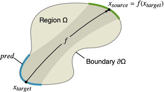
周期境界条件が指定されるかもしれない位置が青で示されている．示された位置は領域Ωの境界∂Ω上にあり，その位置の解と緑で示された位置の解との関係を指定する．関数 f は青の位置から緑の位置にマップする．
矩形領域Ωの特殊ケースでは，境界方程式 u[…,x_i,min,…]u[…,x_i,max,…]がPeriodicBoundaryCondition[u[…,x_i,…],x_ix_i,max,f]と等しいとみなされる．ただし，f=TranslationTransform[{…,0,x_i,min-x_i,max,0,…}]である． »
独立変数 x₁,…における方程式と不等式の任意の論理結合を述語 pred に使うことができる．
pred がTrueである∂Ωの一部の任意の点 x_targetについてのPeriodicBoundaryCondition[a+b u[x₁,…],pred,f]では，x_source=f[x_target]は pred がTrueではない∂Ω内の点でなければならない．
NDSolveでPeriodicBoundaryCondition[a+b u[x₁,…],pred,f]のとき，系の行列は解の値 u[x_target]が pred がTrueであるΩの境界上のすべての x_targetについて u[x_source]==a+b u[x_target]をほぼ満足するようなに変形される．
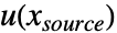についての陰的ノイマン零点条件を含む境界条件もまた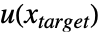，にマッピングされる．
PeriodicBoundaryCondition[a+b u[x₁,…],pred,f]では，a と b の両方が時間を含む任意の独立変数 x_iに依存するかもしれないスカラー値である．
反周期的境界はPeriodicBoundaryCondition[-u[x₁,…],pred,f]を使って指定できる．
aとbのよく使われるあたいには以下がある．

	u[x₁,…]	周期境界条件
	-u[x₁,…]	反周期境界条件
	a u[x₁,…]	スケールされた周期境界条件
	u[x₁,…]+b	オフセット周期境界条件

PeriodicBoundaryConditionは，有限要素近似については，1Dのノード，2Dの辺，3Dの面に作用する．

例題

すべて開くすべて閉じる

例 (2)

周期境界条件を持つラプラシアンの5つの固有値と固有ベクトルを求める：

Wolfram Language code:

{vals, funs} = NDEigensystem[{-u''[x], PeriodicBoundaryCondition[u[x], x == 2π, Function[X, X - 2π]]}, u[x], {x, 0, 2π}, 5];

求まった固有値を期待される解析的固有値と比較する：

Wolfram Language code: vals - Flatten[Join[{0}, Table[{n ^ 2, n ^ 2}, {n, 1, 2}]]]

固有関数を可視化する：

Wolfram Language code: Plot[funs, {x, 0, 2π}]

境界が周期的かどうか調べる：

Wolfram Language code: (funs /. x -> 0) - (funs /. x -> 2π)

曲線的境界上に周期境界条件を持つポアソン(Poisson)方程式を解く：

Wolfram Language code: Ω = RegionDifference[RegionUnion[Disk[], Rectangle[{0, -1}, {2, 1}]], Disk[{2, 0}]];

Wolfram Language code:

ufun = NDSolveValue[{-Subsuperscript[∇, {x, y}, 2]u[x, y] == If[(x - 1 / 4) ^ 2 + y ^ 2 ≤ 1 / 4, 1, 0], PeriodicBoundaryCondition[u[x, y], x ^ 2 + y ^ 2 == 1, Function[X, X + {2, 0}]], DirichletCondition[u[x, y] == 0, (10 ^ -14 < x < 2 && (y == -1 || y == 1))]}, u, {x, y}∈Ω];

解を可視化する：

Wolfram Language code: cp = ContourPlot[ufun[x, y], {x, y}∈Ω, ColorFunction -> "TemperatureMap", AspectRatio -> Automatic]

周期解を可視化する：

Wolfram Language code: Show[MapAt[Translate[#, {2, 0}]&, cp, 1], cp, MapAt[Translate[#, {-2, 0}]&, cp, 1], PlotRange -> All]

スコープ (15)

1D固有値問題 (7)

マシュー(Mathieu)方程式の5つの固有値と固有ベクトルを求める：

Wolfram Language code:

{vals, funs} = NDEigensystem[{-u''[x] + 4 Cos[2x] u[x], PeriodicBoundaryCondition[u[x], x == 2π, Function[X, X - 2π]]}, u[x], {x, 0, 2π}, 5];

固有関数を可視化する：

Wolfram Language code: Plot[funs, {x, 0, 2π}]

境界が周期的かどうかを調べる：

Wolfram Language code: (funs /. x -> 0) - (funs /. x -> 2π)

これは等価である：

Wolfram Language code:

{vals, funs} = NDEigensystem[{-u''[x] + 4 Cos[2x] u[x], u[0] == u[2π]}, u[x], {x, 0, 2π}, 5];
(funs /. x -> 0) - (funs /. x -> 2π)

反周期的境界を持つラプラシアンの5つの固有値と固有ベクトルを求める：

Wolfram Language code:

{vals, funs} = NDEigensystem[{-u''[x], PeriodicBoundaryCondition[-u[x], x == 2π, TranslationTransform[{-2π}]]}, u[x], {x, 0, 2π}, 5];

固有値を調べる：

Wolfram Language code: vals

固有関数を可視化する：

Wolfram Language code: Plot[funs, {x, 0, 2π}]

端点で固有ベクトルの計算が合うことを調べる：

Wolfram Language code: Plus[funs /. x -> 0, funs /. x -> 2π]

細かいメッシュ上でマイスナー(Meissner)方程式の9つの固有値と固有ベクトルを求める：

Wolfram Language code:

w[x_] := If[x < 0, 1, 9]
{vals, funs} = NDEigensystem[{-1 / w[x]u''[x], PeriodicBoundaryCondition[u[x], x == 1 / 2, TranslationTransform[{-1}]]}, u[x], {x, -1 / 2, 1 / 2}, 9, Method -> {
	"SpatialDiscretization" -> {"FiniteElement", {"MeshOptions" -> {MaxCellMeasure -> 0.001}}}
	}];

固有値を期待される解析的固有値と比較する：

Wolfram Language code:

α = ArcCos[-7 / 8];
vals - Join[{0}, Flatten[Table[{(2 * n * π + α) ^ 2, (2 * (n + 1) * π - α) ^ 2, (2 * (n + 1) * π) ^ 2, (2 * (n + 1) * π) ^ 2}, {n, 0, 1}]]]

固有関数を可視化する：

Wolfram Language code: Plot[funs, {x, -1 / 2, 1 / 2}]

対称ポテンシャルがあるSturm–Liouville演算子の5つの固有値と固有ベクルを求める：

Wolfram Language code:

V[x_] := Cos[x];
{vals, funs} = NDEigensystem[{-u''[x] - (V''[x] - V'[x] ^ 2) u[x], PeriodicBoundaryCondition[u[x], x == 2π, TranslationTransform[{-2π}]]}, u[x], {x, 0, 2π}, 5];

固有値を調べる：

Wolfram Language code: vals

固有値をより高い解像度で再計算する：

Wolfram Language code:

{vals, funs} = NDEigensystem[{-u''[x] - (V''[x] - V'[x] ^ 2) u[x], PeriodicBoundaryCondition[u[x], x == 2π, TranslationTransform[{-2π}]]}, u[x], {x, 0, 2π}, 5, Method -> {"SpatialDiscretization" -> {"FiniteElement", "MeshOptions" -> {"MaxCellMeasure" -> 0.001}}}];

Wolfram Language code: vals

固有関数を可視化する：

Wolfram Language code: Plot[funs, {x, 0, 2π}]

非対称ポテンシャルを持つSturm–Liouville演算子の5つの周期的固有値と固有ベクトルを求める：

Wolfram Language code:

V[x_] := Cos[x] + x;
{vals, funs} = NDEigensystem[{-u''[x] - (V''[x] - V'[x] ^ 2) u[x], PeriodicBoundaryCondition[u[x], x == 2π, TranslationTransform[{-2π}]]}, u[x], {x, 0, 2π}, 5];

固有値を調べる：

Wolfram Language code: vals

固有関数を可視化する：

Wolfram Language code: Plot[funs, {x, 0, 2π}]

非対称ポテンシャルを持つSturm–Liouville演算子の5つの反周期的固有値と固有ベクトルを求める：

Wolfram Language code:

V[x_] := Cos[x] + x;
{vals, funs} = NDEigensystem[{-u''[x] - (V''[x] - V'[x] ^ 2) u[x], PeriodicBoundaryCondition[-u[x], x == 2π, TranslationTransform[{-2π}]]}, u[x], {x, 0, 2π}, 5];

固有値を調べる：

Wolfram Language code: vals

固有関数を可視化する：

Wolfram Language code: Plot[funs, {x, 0, 2π}]

端点で固有ベクトルの計算が合うことを調べる：

Wolfram Language code: Plus[funs /. x -> 0, funs /. x -> 2π]

反対称ポテンシャルを持つSturm–Liouville演算子の5つの相関的反周期的固有値と固有ベクトルを求める：

Wolfram Language code:

V[x_] := Cos[x] + x;
{vals, funs} = NDEigensystem[{-u''[x] - (V''[x] - V'[x] ^ 2) u[x], PeriodicBoundaryCondition[-2u[x], x == 2π, TranslationTransform[{-2π}]]}, u[x], {x, 0, 2π}, 5];

固有値を調べる：

Wolfram Language code: vals

固有関数を可視化する：

Wolfram Language code: Plot[funs, {x, 0, 2π}]

固有値が端点で関係と一致することを調べる：

Wolfram Language code: (funs /. x -> 0) - (-2) * (funs /. x -> 2π)

1Dと時間偏微分方程式の問題 (2)

周期境界条件を持つ1Dのシュレディンガー(Schrödinger)方程式を解く：

Wolfram Language code:

ufun = NDSolveValue[{I D[u[t, x], t] == -D[u[t, x], {x, 2}], u[0, x] == Exp[-(x ^ 2)], 
	PeriodicBoundaryCondition[u[t, x], x == -5, TranslationTransform[{10}]]
	}, u, {t, 0, 5}, {x}∈Line[{{-5}, {5}}]]

波動関数を可視化する：

Wolfram Language code:

plots = Table[Plot[Abs[ufun[t, x]], {x, -5, 5}, PlotRange -> {0, 1}], {t, 0, 3, .1}];
ListAnimate[plots]

周期的境界条件を持つ1Dの波動方程式を解く：

Wolfram Language code:

f[x_] = D[0.125 Erf[(x - 0.5) / 0.125], x];
vInit[x_] = -D[f[x], x];
ufun = NDSolveValue[{D[u[t, x], {t, 2}] - D[u[t, x], {x, 2}] == NeumannValue[-Derivative[1, 0][u][t, x], x == 0 || x == 1]
	, u[0, x] == f[x]
	, Derivative[1, 0][u][0, x] == vInit[x]
	, PeriodicBoundaryCondition[u[t, x], x == 0, TranslationTransform[{1}]]
	}, u, {t, 0, 2}, {x, 0, 1}];

周期的波動関数を可視化する：

Wolfram Language code:

plots = Table[Plot[ufun[t, x], {x, 0, 1}], {t, 0, 2, .1}];
ListAnimate[plots]

上記の例ではがターゲットとして使われている．この場合，ターゲットは流束が周期領域に入るところに置かれている．

代りにがターゲットなら，に達すると波パルスが反転して逆方向に進む．で陰的ノイマン(Neumann)ゼロ境界条件がハード境界条件を強制し，パルスはそのハード境界を反射する：

Wolfram Language code:

ufunM = NDSolveValue[{D[u[t, x], {t, 2}] - D[u[t, x], {x, 2}] == NeumannValue[-Derivative[1, 0][u][t, x], x == 0 || x == 1]
	, u[0, x] == f[x]
	, Derivative[1, 0][u][0, x] == vInit[x]
	, PeriodicBoundaryCondition[u[t, x], x == 1, TranslationTransform[{-1}]]
	}, u, {t, 0, 2}, {x, 0, 1}];

2つの周期波動関数を比較する：

Wolfram Language code:

plots = Table[Plot[{ufun[t, x], ufunM[t, x]}, {x, 0, 1}, PlotRange -> 1.15, PlotLegends -> LineLegend[{"x=0", "x=1"}, LegendLabel -> "target"]], 
	{t, 0, 2, .1}];
ListAnimate[plots]

2D偏微分方程式の問題 (4)

DirichletConditionを使って上下で偏微分方程式を解くための矩形の領域を設定する：

Wolfram Language code:

Ω = Rectangle[{0, 0}, {2, 1}];
pde = -Subsuperscript[∇, {x, y}, 2]u[x, y] == If[1.25 ≤ x ≤ 1.75 && 0.25 ≤ y ≤ 0.5, 1., 0.];
Subscript[Γ, D] = DirichletCondition[u[x, y] == 0, (y == 0 || y == 1) && 0 < x ≤ 2];

周期境界条件を実装するために，ターゲット(x==0) からソース(x==2)までのマッピング f を指定する：

Wolfram Language code: f = TranslationTransform[{2, 0}];

周期境界条件の領域Ωとソースを緑で，ターゲットを青で可視化する：

Wolfram Language code:

Show[RegionPlot[Ω], Graphics[{Thickness[0.015], #}]& /@ {{Darker[Green], TransformedRegion[#, f]}, {Darker[Blue], #}}&[Line[{{0, 0}, {0, 1}}]], AspectRatio -> Automatic]

マッピング関数 f を使って周期境界条件を指定する：

Wolfram Language code: pbc = PeriodicBoundaryCondition[u[x, y], x == 0, f];

方程式を解き，可視化する：

Wolfram Language code:

ufun = NDSolveValue[{pde, pbc, Subscript[Γ, D]}, u, {x, y}∈Ω];
ContourPlot[ufun[x, y], {x, y}∈Ω, ColorFunction -> "TemperatureMap", AspectRatio -> Automatic]

左下のコーナーにDirichletConditionがあり周期境界条件で反対側とリンクされた矩形の上でラプラス型の方程式の解を求める：

Wolfram Language code:

ufun = NDSolveValue[{-Laplacian[u[x, y], {x, y}] == 10 x ^ 5 * y ^ 3, 
	DirichletCondition[u[x, y] == 0, x == 0 && y == 0], PeriodicBoundaryCondition[u[x, y], 0 ≤ y ≤ 1 && x == 1, FindGeometricTransform[{{0, 0}, {0, 1}}, {{1, 0}, {1, 1}}][[2]]], PeriodicBoundaryCondition[u[x, y], 0 ≤ x ≤ 1 && y == 1, FindGeometricTransform[{{0, 0}, {1, 0}}, {{0, 1}, {1, 1}}][[2]]]}, u, {x, y}∈Rectangle[{0, 0}, {1, 1}]];

結果を可視化する：

Wolfram Language code: Plot3D[ufun[x, y], {x, y}∈Rectangle[{0, 0}, {1, 1}]]

境界における解の差を調べる：

Wolfram Language code: GraphicsColumn[{Plot[ufun[x, 0] - ufun[x, 1], {x, 0, 1}], Plot[ufun[0, y] - ufun[1, y], {y, 0, 1}]}]

左下コーナーのDirichletConditionが他のコーナーにも伝播していることに注意のこと：

Wolfram Language code: {ufun[0, 0], ufun[1, 0], ufun[0, 1], ufun[1, 1]}

領域を指定する：

Wolfram Language code: Ω = ImplicitRegion[1 ≤ x ^ 2 + y ^ 2 ≤ 4 && x - y ≥ 0 && x ≥ 0 && y ≥ 0, {x, y}];

領域と境界を示す：

Wolfram Language code:

Show[RegionPlot[Ω], ContourPlot[{-y == 0, 1 - x ^ 2 - y ^ 2 == 0, -4 + x ^ 2 + y ^ 2 == 0, -x + y == 0}, {x, 1 / Sqrt[2] - .1, 2 + .1}, {y, -.1, Sqrt[2] + .1}, ContourStyle -> {Darker[Green], Orange, Orange, Darker[Blue]}], AspectRatio -> Automatic, PlotRange -> {{0.6, 2.1}, {-0.1, 1.5}}]

ターゲット（青）からソース（緑）にマップするマッピング f を求める：

Wolfram Language code: {error, f} = FindGeometricTransform[{{1, 0}, {2, 0}}, {{1 / Sqrt[2], 1 / Sqrt[2]}, {Sqrt[2], Sqrt[2]}}];

内部発熱があり，オレンジ色の境界の温度が固定されていて，周期境界条件が緑のソースと青のターゲット境界をリンクしているポアソン方程式を解く：

Wolfram Language code:

ufun = NDSolveValue[{-Subsuperscript[∇, {x, y}, 2]u[x, y] == If[1.4 ≤ x ≤ 1.6 && 0 ≤ y ≤ 0.1, 1., 0.], PeriodicBoundaryCondition[u[x, y], (y - x) == 0, f], DirichletCondition[u[x, y] == 0, (x ^ 2 + y ^ 2 == 1 || x ^ 2 + y ^ 2 == 4) && !(y - x) > -10 ^ -7]}, u, {x, y}∈Ω];

周期境界が同じ値を持つことを調べる：

Wolfram Language code: Plot[{ufun[x, 0] - ufun@@InverseFunction[f][{x, 0}]}, {x, 1, 2}, PlotRange -> All]

解を可視化する：

Wolfram Language code: ContourPlot[ufun[x, y], {x, y}∈Ω, ColorFunction -> "TemperatureMap", Contours -> 21]

反周期的解と比較する：

Wolfram Language code:

ufun = NDSolveValue[{-Subsuperscript[∇, {x, y}, 2]u[x, y] == If[1.4 ≤ x ≤ 1.6 && 0 ≤ y ≤ 0.1, 1., 0.], PeriodicBoundaryCondition[-u[x, y], (y - x) == 0, f], DirichletCondition[u[x, y] == 0, (x ^ 2 + y ^ 2 == 1 || x ^ 2 + y ^ 2 == 4) && !(y - x) > -10 ^ -7]}, u, {x, y}∈Ω];
ContourPlot[ufun[x, y], {x, y}∈Ω, ColorFunction -> "TemperatureMap", Contours -> 21]

領域を指定する：

Wolfram Language code:

Ω = Rectangle[{0, 0}, {2, 1}];
pde = -Subsuperscript[∇, {x, y}, 2]u[x, y] == If[1.25 ≤ x ≤ 1.75 && 0.25 ≤ y ≤ 0.5, 1., 0.];

上下の部分はDirichletConditionに従う：

Wolfram Language code: Subscript[Γ, D] = DirichletCondition[u[x, y] == 0, (y == 0 || y == 1) && 0 < x ≤ 2];

左側の辺は右側の辺（ソース）相対的境界条件のターゲットである：

Wolfram Language code:

a = -1 / 20;b = 2;
pbc = PeriodicBoundaryCondition[a + b * u[x, y], x == 0 && 0 ≤ y ≤ 1, TranslationTransform[{2, 0}]];

方程式を解き，可視化する：

Wolfram Language code:

ufun = NDSolveValue[{pde, pbc, Subscript[Γ, D]}, u, {x, y}∈Ω];
ContourPlot[ufun[x, y], {x, y}∈Ω, ColorFunction -> "TemperatureMap", AspectRatio -> Automatic]

周期境界が正しい関係にあることを調べる：

Wolfram Language code: Plot[{a + b * ufun[0, y] - ufun[2, y]}, {y, 0, 1}, PlotRange -> All]

2Dと時間の偏微分方程式の問題 (1)

ボックスへの適合ポテンシャルと周期境界条件を持つ時間依存の2Dシュレディンガー方程式を解く：

Wolfram Language code:

ufun = NDSolveValue[{I D[u[t, x, y], t] == -D[u[t, x, y], {x, 2}] - D[u[t, x, y], {y, 2}] - 20 Cos[Pi x / 10] Cos[Pi y / 10] u[t, x, y], u[0, x, y] == Exp[-((x - 1) ^ 2 + y ^ 2)] Exp[I y], PeriodicBoundaryCondition[u[t, x, y], x == -5, TranslationTransform[{10, 0}]], 
	PeriodicBoundaryCondition[u[t, x, y], y == -5, TranslationTransform[{0, 10}]]}, u, {t, 0, 3}, {x, y}∈Rectangle[{-5, -5}, {5, 5}]];

波動関数を可視化する：

Wolfram Language code:

plots = Table[Plot3D[Abs[ufun[t, x, y]], {x, -5, 5}, {y, -5, 5}, PlotRange -> {0, 1}], {t, 0, 3, .1}];
ListAnimate[plots]

3Dの問題 (1)

周期境界条件がある直方体内でポアソン方程式を解く：

Wolfram Language code: Ω = Cuboid[{0, 0, 0}, {5, 1, 1}];

Wolfram Language code:

ufun = NDSolveValue[{-Laplacian[u[x, y, z], {x, y, z}] == 1, DirichletCondition[u[x, y, z] == 0, 0 < x < 5], PeriodicBoundaryCondition[u[x, y, z], x == 0, TranslationTransform[{5, 0, 0}]]}, u, {x, y, z}∈Ω]

解を可視化する：

Wolfram Language code:

SliceContourPlot3D[ufun[x, y, z], {{"XStackedPlanes", {0, 1.5, 3.5, 5}}, {"YStackedPlanes", 1}, {"ZStackedPlanes", 1}}, {x, y, z}∈Ω, ColorFunction -> "TemperatureMap", Boxed -> False, Axes -> False]

アプリケーション (1)

Disk上のLaplacianの固有値を極座標で計算する：

Wolfram Language code:

pvals = NDEigenvalues[{-Laplacian[u[r, ϕ], {r, ϕ}, "Polar"], DirichletCondition[u[r, ϕ] == 0, r == 1 && 0 < ϕ ≤ 2π], PeriodicBoundaryCondition[u[r, ϕ], ϕ == 0, TranslationTransform[{0, 2 π}]]}, u[r, ϕ], {r, 0, 1}, {ϕ, 0, 2π}, 3]

Disk上のLaplacianの固有値を直交座標で解析的に計算する：

Wolfram Language code: avals = DEigenvalues[{-Laplacian[u[x, y], {x, y}], DirichletCondition[u[x, y] == 0, True]}, u[x, y], {x, y}∈Disk[], 3]

計算された固有値を比較する：

Wolfram Language code: pvals - avals

Disk上のLaplacianの固有値を直交座標で数値的に計算する：

Wolfram Language code:

cvals = NDEigenvalues[{-Laplacian[u[x, y], {x, y}], DirichletCondition[u[x, y] == 0, True]}, u[x, y], {x, y}∈Disk[], 3]

直交座標で数値的に計算された固有値を解析解と比較する：

Wolfram Language code: cvals - avals

数値的に計算された固有値を比較する：

Wolfram Language code: cvals - pvals

考えられる問題 (8)

定常偏微分方程式に周期境界条件だけを指定すると，一意的ではない解が求まることがある．場合によっては系が非可解のことがある：

Wolfram Language code:

V[x_] := Cos[x];
ufun = NDSolveValue[{u''[x] + (V''[x] - V'[x] ^ 2) u[x] == -1, 
	PeriodicBoundaryCondition[u[x], x == 2π, TranslationTransform[{-2 π}]]}, u, {x, 0, 2π}]

Wolfram Language code: Plot[ufun[x], {x, 0, 2π}]

ソースの境界にDirichletConditionを指定する：

Wolfram Language code:

V[x_] := Cos[x];
ufun = NDSolveValue[{u''[x] + (V''[x] - V'[x] ^ 2) u[x] == -1, 
	DirichletCondition[u[x] == 0, x == 0], 
	PeriodicBoundaryCondition[u[x], x == 2π, TranslationTransform[{-2 π}]]}, u, {x, 0, 2π}]

Wolfram Language code: Plot[ufun[x], {x, 0, 2π}]

PeriodicBoundaryConditionのマッピング f のソースは領域の境界上にある必要はない：

Wolfram Language code:

domain = {x, 0, 2π};
f1 = TranslationTransform[{-π}];

Wolfram Language code:

V[x_] := Cos[x];
ufun = NDSolveValue[{u''[x] + (V''[x] - V'[x] ^ 2) u[x] == -1, 
	DirichletCondition[u[x] == 0, x == 0], 
	PeriodicBoundaryCondition[u[x], x == 2π, f1]}, u, domain]

結果を可視化する：

Wolfram Language code: Plot[ufun[x], {x, 0, 2π}]

であることに注意のこと：

Wolfram Language code: ufun[f1[{2π}]] - ufun[2π]

ソースが境界上にある解と比較する：

Wolfram Language code: f2 = TranslationTransform[{-2π}];

Wolfram Language code:

V[x_] := Cos[x];
ufun = NDSolveValue[{u''[x] + (V''[x] - V'[x] ^ 2) u[x] == -1, 
	DirichletCondition[u[x] == 0, x == 0], 
	PeriodicBoundaryCondition[u[x], x == 2π, f2]}, u, {x, 0, 2π}]

結果を可視化する：

Wolfram Language code: Plot[ufun[x], {x, 0, 2π}]

DirichletConditionはターゲットの境界上にあってはならない：

Wolfram Language code:

V[x_] := Cos[x];
ufun = NDSolveValue[{u''[x] + (V''[x] - V'[x] ^ 2) u[x] == -1, 
	DirichletCondition[u[x] == 0, x == 2π], 
	PeriodicBoundaryCondition[u[x], x == 2π, TranslationTransform[{-2 π}]]}, u, {x, 0, 2π}]

DirichletConditionをソースの境界に移動するとうまくいく：

Wolfram Language code:

V[x_] := Cos[x];
ufun = NDSolveValue[{u''[x] + (V''[x] - V'[x] ^ 2) u[x] == -1, 
	DirichletCondition[u[x] == 0, x == 0], 
	PeriodicBoundaryCondition[u[x], x == 2π, TranslationTransform[{-2 π}]]}, u, {x, 0, 2π}, Method -> "FiniteElement"]

周期境界条件は偏微分方程式の解をソースからターゲットの境界に伝播する．どの境界をソースとみなしどれをターゲットとみなすかの選択は，偏微分方程式の解に影響する．

矩形領域と非対称ポアソン方程式について考える：

Wolfram Language code:

Ω = Rectangle[{0, 0}, {2, 1}];
pde = -Subsuperscript[∇, {x, y}, 2]u[x, y] == If[1.25 ≤ x ≤ 1.75 && 0.25 ≤ y ≤ 0.5, 1., 0.];

上部と下部DirichletConditionに従う：

Wolfram Language code: Subscript[Γ, D] = DirichletCondition[u[x, y] == 0, (y == 0 || y == 1) && 0 < x ≤ 2];

左側の辺が右側の辺（ソース）のターゲットの境界である：

Wolfram Language code: pbc = PeriodicBoundaryCondition[u[x, y], x == 0 && 0 ≤ y ≤ 1, TranslationTransform[{2, 0}]];

方程式を解き，可視化する：

Wolfram Language code:

ufun = NDSolveValue[{pde, pbc, Subscript[Γ, D]}, u, {x, y}∈Ω];
ContourPlot[ufun[x, y], {x, y}∈Ω, ColorFunction -> "TemperatureMap", AspectRatio -> Automatic]

周期境界における値を調べる：

Wolfram Language code: Plot[{ufun[0, y] - ufun[2, y]}, {y, 0, 1}, PlotRange -> All]

2番目の例では，右側の辺が左側の辺（ソース）のターゲットの境界である：

Wolfram Language code:

Subscript[Γ, D] = DirichletCondition[u[x, y] == 0, (y == 0 || y == 1) && 0 ≤ x < 2];
pbc = PeriodicBoundaryCondition[u[x, y], x == 2 && 0 ≤ y ≤ 1, TranslationTransform[{-2, 0}]];

方程式を解き，可視化する：

Wolfram Language code:

ufun = NDSolveValue[{pde, pbc, Subscript[Γ, D]}, u, {x, y}∈Ω];
ContourPlot[ufun[x, y], {x, y}∈Ω, ColorFunction -> "TemperatureMap", AspectRatio -> Automatic]

周期境界における値を調べる：

Wolfram Language code: Plot[{ufun[0, y] - ufun[2, y]}, {y, 0, 1}, PlotRange -> All]

周期境界条件は偏微分方程式の解をソース領域からターゲット領域に伝播する．マッピングの方向は偏微分方程式の解に影響する．

矩形領域と非対称ポアソン方程式について考える：

Wolfram Language code:

Ω = Rectangle[{0, 0}, {2, 1}];
pde = -Subsuperscript[∇, {x, y}, 2]u[x, y] == If[1.5 ≤ x ≤ 2 && 0 ≤ y ≤ 0.25, 1., 0.];

上部と下部はDirichletConditionに従う：

Wolfram Language code: Subscript[Γ, D] = DirichletCondition[u[x, y] == 0, (y == 0 || y == 1) && 0 < x ≤ 2];

右下を左上にマップし，右上を左下の辺にマップする：

Wolfram Language code: mapping = FindGeometricTransform[{{2, 1}, {2, 0}}, {{0, 0}, {0, 1}}][[2]];

左側の辺は右側の辺のターゲット境界である：

Wolfram Language code: pbc = PeriodicBoundaryCondition[u[x, y], x == 0 && 0 ≤ y ≤ 1, mapping];

方程式を解き，可視化する：

Wolfram Language code:

ufun = NDSolveValue[{pde, pbc, Subscript[Γ, D]}, u, {x, y}∈Ω];
ContourPlot[ufun[x, y], {x, y}∈Ω, ColorFunction -> "TemperatureMap", AspectRatio -> Automatic]

辺を入れ替えた同方向へのマッピングを比較する．右下から左下と右上から左上へ：

Wolfram Language code: mapping = FindGeometricTransform[{{2, 0}, {2, 1}}, {{0, 0}, {0, 1}}][[2]];

左側は右側のターゲット境界である：

Wolfram Language code: pbc = PeriodicBoundaryCondition[u[x, y], x == 0 && 0 ≤ y ≤ 1, mapping];

方程式を解き，可視化する：

Wolfram Language code:

ufun = NDSolveValue[{pde, pbc, Subscript[Γ, D]}, u, {x, y}∈Ω];
ContourPlot[ufun[x, y], {x, y}∈Ω, ColorFunction -> "TemperatureMap", AspectRatio -> Automatic]

周期境界条件は，ソースからの偏微分方程式の解をターゲットの境界に関連させる．ソースにおける境界条件は，これもまた陰的なものだが，ターゲットにおける解に影響する．

この動作の例として，有限要素法で離散化された時間依存方程式について考える．初期条件 u と陰的なノイマンゼロ境界条件が両方に指定されており，PeriodicBoundaryConditionは指定されていない：

Wolfram Language code:

ufun = NDSolveValue[{D[u[t, x], t] - D[u[t, x], {x, 2}] == 0, u[0, x] == Sin[x]}, u, {t, 0, 1}, {x, -π, π}, Method -> {"MethodOfLines", "SpatialDiscretization" -> {"FiniteElement"}}]

さまざまな時点における解を可視化する：

Wolfram Language code:

frames = Table[Plot[ufun[t, x], {x, -π, π}, PlotRange -> {-1, 1}], {t, 0, 1, 0.1}];
ListAnimate[frames, SaveDefinitions -> True]

両方の空間的境界で，陰的ノイマンゼロ境界条件が満足されることに注意のこと．

陰的ノイマン0境界条件を持つソースの境界にPeriodicBoundaryConditionが使われると，その条件がターゲットの境界にマップされる．

次は，前と同じ方程式の解および初期条件と，左辺にソース右辺にターゲットを持つ追加的な周期境界条件である：

Wolfram Language code:

ufun = NDSolveValue[{D[u[t, x], t] - D[u[t, x], {x, 2}] == 0, u[0, x] == Sin[x], PeriodicBoundaryCondition[u[t, x], x == π, Function[X, X - 2π]]}, u, {t, 0, 1}, {x, -π, π}, Method -> {"MethodOfLines", "SpatialDiscretization" -> {"FiniteElement"}}]

さまざまな時点における解を可視化する：

Wolfram Language code:

frames = Table[Plot[ufun[t, x], {x, -π, π}, PlotRange -> {-1, 1}], {t, 0, 1, 0.1}];
ListAnimate[frames, SaveDefinitions -> True]

左辺の陰的ノイマン0境界条件における解の値がどのように右辺にマップされるかに注意のこと．

これは有限要素法では予想される動作である．テンソル積格子メソッドは陰的境界条件を持たないので異なる動作を示す：

Wolfram Language code:

ufunTPG = NDSolveValue[{D[u[t, x], t] - D[u[t, x], {x, 2}] == 0, u[0, x] == Sin[x], u[t, -π] == u[t, π]}, u, {t, 0, 1}, {x, -π, π}, Method -> {"MethodOfLines", "SpatialDiscretization" -> {"TensorProductGrid"}}]

さまざまな時点におけるテンソル積格子解を可視化する：

Wolfram Language code:

frames = Table[Plot[ufunTPG[t, x], {x, -π, π}, PlotRange -> {-1, 1}], {t, 0, 1, 0.1}];
ListAnimate[frames, SaveDefinitions -> True]

左辺にDirichletConditionを指定し，PeriodicBoundaryConditionを指定すると有限要素法でも同様の動作を得ることができる：

Wolfram Language code:

ufunFEM = NDSolveValue[{D[u[t, x], t] - D[u[t, x], {x, 2}] == 0, u[0, x] == Sin[x], PeriodicBoundaryCondition[u[t, x], x == π, Function[X, X - 2π]], DirichletCondition[u[t, x] == Sin[-π], x == -π]}, u, {t, 0, 1}, {x, -π, π}, Method -> {"MethodOfLines", "SpatialDiscretization" -> {"FiniteElement"}}]

さまざまな時点における有限要素とテンソル積の格子解の差を可視化する：

Wolfram Language code:

frames = Table[Plot[ufunFEM[t, x] - ufunTPG[t, x], {x, -π, π}, PlotRange -> {-5 10 ^ -4, 5 10 ^ -4}], {t, 0, 1, 0.1}];
ListAnimate[frames, SaveDefinitions -> True]

代替策として，各辺にDirichletConditionを指定することもできる．

周期境界条件はソースからの偏微分方程式の解をターゲットの境界と関連付ける．ソースにおける境界条件は，陰的なものも含め，ターゲントの解に影響する．複数の周期境界条件を使って連続導関数を強制することができる．

領域と周期境界条件を引数として取るヘルパー関数を設定する：

Wolfram Language code:

Ω = Rectangle[{0, 0}, {2, 1}];
fun[pbcs__] := NDSolveValue[{-Laplacian[u[x, y], {x, y}] == If[(1.25 ≤ x + 2 ≤ 1.75 || 1.25 ≤ x ≤ 1.75) && 0.25 ≤ y ≤ 0.5, 1., 0.], 
	pbcs, 
	DirichletCondition[u[x, y] == 0, (y == 0 || y == 1) && 0 < x < 2]}, u, {x, y}∈Ω, Method -> {"FiniteElement", "MeshOptions" -> {"MaxCellMeasure" -> 0.0001, "MeshElementType" -> TriangleElement}}];

プロットオプションとヘルパー関数を設定して周期プロットを作成する：

Wolfram Language code:

opts = {PlotRange -> All, AspectRatio -> Automatic, ColorFunction -> "TemperatureMap", Frame -> {True, True}, PlotRangePadding -> None, ImageSize -> Large};
periodicPlot[cp_] := Show[MapAt[Translate[#, {2, 0}]&, cp, 1], cp, MapAt[Translate[#, {-2, 0}]&, cp, 1], PlotRange -> All]

左側に単一の周期境界条件を持つ偏微分方程式を解く：

Wolfram Language code: ufun = fun[PeriodicBoundaryCondition[u[x, y], x == 0 && 0 ≤ y ≤ 1, TranslationTransform[{2, 0}]]];

解の周期等高線プロットを可視化する：

Wolfram Language code: periodicPlot[ContourPlot[ufun[x, y], {x, y}∈Ω, Evaluate[opts]]]

解の傾きの周期流線密度プロットを可視化する：

Wolfram Language code:

periodicPlot[StreamDensityPlot[Evaluate@{-Grad[ufun[x, y], {x, y}], ufun[x, y]}, {x, y}∈Ω, StreamScale -> Tiny, Evaluate[opts]]]

傾きは連続的ではない点に注意のこと．これは，ソースの位置に存在する陰的ノイマン値のためである．

同様に，解の傾きのノルムの周期密度プロットを可視化する：

Wolfram Language code: periodicPlot[DensityPlot[Evaluate[Norm@Grad[ufun[x, y], {x, y}]], {x, y}∈Ω, Evaluate[opts]]]

2番目の周期境界条件を指定すると連続導関数が強制される．左側と右側の両方に周期境界条件がある偏微分方程式を解く：

Wolfram Language code:

ufun = fun[PeriodicBoundaryCondition[u[x, y], x == 0 && 0 ≤ y ≤ 1, TranslationTransform[{2, 0}]], PeriodicBoundaryCondition[u[x, y], x == 2 && 0 ≤ y ≤ 1, TranslationTransform[{-2, 0}]]];

解の周期等高線プロットを可視化する．予想されるように，解は変化していて陰的ノイマン値が除去されている：

Wolfram Language code: periodicPlot[ContourPlot[ufun[x, y], {x, y}∈Ω, Evaluate[opts]]]

解の傾きの周期流線密度プロットを可視化する．傾きが連続的になっている点に注意のこと：

Wolfram Language code:

periodicPlot[StreamDensityPlot[Evaluate@{-Grad[ufun[x, y], {x, y}], ufun[x, y]}, {x, y}∈Ω, StreamScale -> Tiny, Evaluate[opts]]]

同様に解の傾きのノルムの周期密度プロットを可視化して，傾きのノルムもまた連続的であることを確認する：

Wolfram Language code: periodicPlot[DensityPlot[Evaluate[Norm@Grad[ufun[x, y], {x, y}]], {x, y}∈Ω, Evaluate[opts]]]

この手法は非構造化メッシュでも使うことができる．

ノイマン値のような周期境界条件は，2Dの辺と3Dの面に作用する．これは，周期境界条件が作用するためには有限要素メッシュに十分なノードがなければならないことを意味する．

有限要素メッシュを生成し，メッシュのノードを可視化する：

Wolfram Language code:

mesh = NDSolve`FEM`ToElementMesh["Coordinates" -> {{0., 0.}, {0.25, 0.}, {0.5, 0.}, {0.75, 0.}, {1., 0.}, {0., 0.5}, {0.25, 0.5}, {0.5, 0.5}, {0.75, 0.5}, {1., 0.5}, {0., 1.}, {0.25, 1.}, {0.5, 1.}, {0.75, 1.}, {1., 1.}}, "MeshElements" -> {NDSolve`FEM`QuadElement[{{1, 2, 7, 6}, {2, 3, 8, 7}, {3, 4, 9, 8}, {4, 5, 10, 9}, {6, 7, 12, 11}, {7, 8, 13, 12}, {8, 9, 14, 13}, {9, 10, 15, 14}}]}];
Show[
	mesh["Wireframe"], 
	mesh["Wireframe"["MeshElement" -> "PointElements", "MeshElementIDStyle" -> LightDarkSwitched[Black, White]]]]

単一の点をマッピングする周期境界条件で偏微分方程式を解く：

Wolfram Language code:

pde = Laplacian[u[x, y], {x, y}] == 0;
bc = DirichletCondition[u[x, y] == (x - 1 / 2) ^ 2, Or[x == 1, x < 0.5]];
NDSolveValue[{pde, bc
	, PeriodicBoundaryCondition[u[x, y], 0.5 < x < 1, Function[X, X - {1, 0}]]
	}, u, Element[{x, y}, mesh]]

これを修正するために，辺を被覆する周期境界条件のための述語を指定する：

Wolfram Language code:

NDSolveValue[{pde, bc
	, PeriodicBoundaryCondition[u[x, y], 0.5 ≤ x < 1, Function[X, X - {1, 0}]]
	}, u, Element[{x, y}, mesh]]

おもしろい例題 (1)

ボックス上で波動方程式を解くための領域を指定する：

Wolfram Language code: Ω = RegionUnion[Rectangle[{0, 0}, {4, 1}], Rectangle[{1, -1}, {2, 0}], Rectangle[{1, 1}, {2, 2}]];

色で辺をマッチするようなマッピング関数設定する．破線が各ターゲットである：

Wolfram Language code:

f1 = FindGeometricTransform[{{1, 0}, {0, 0}}, {{1, 0}, {1, -1}}][[2]];
f2 = FindGeometricTransform[{{1, -1}, {2, -1}}, {{4, 0}, {3, 0}}][[2]];
f3 = FindGeometricTransform[{{2, 0}, {2, -1}}, {{2, 0}, {3, 0}}][[2]];
f4 = FindGeometricTransform[{{0, 0}, {0, 1}}, {{4, 0}, {4, 1}}][[2]];
f5 = FindGeometricTransform[{{1, 2}, {2, 2}}, {{4, 1}, {3, 1}}][[2]];
f6 = FindGeometricTransform[{{2, 1}, {2, 2}}, {{2, 1}, {3, 1}}][[2]];
f7 = FindGeometricTransform[{{1, 1}, {0, 1}}, {{1, 1}, {1, 2}}][[2]];

細かいメッシュ上で波動方程式を解く：

Wolfram Language code:

ufun = NDSolveValue[{D[u[t, x, y], t, t] == Laplacian[u[t, x, y], {x, y}]
	, u[0, x, y] == Exp[-((x - 3 / 2) ^ 2 + (y - 1 / 2) ^ 2) * 100]
	, Derivative[1, 0, 0][u][0, x, y] == 0
	, PeriodicBoundaryCondition[Derivative[1, 0, 0][u][t, x, y], x == 1 && -1 ≤ y ≤ 0, f1]
	, PeriodicBoundaryCondition[Derivative[1, 0, 0][u][t, x, y], y == 0 && 3 ≤ x ≤ 4, f2]
	, PeriodicBoundaryCondition[Derivative[1, 0, 0][u][t, x, y], y == 0 && 2 ≤ x ≤ 3, f3]
	, PeriodicBoundaryCondition[Derivative[1, 0, 0][u][t, x, y], x == 4 && 0 ≤ y ≤ 1, f4]
	, PeriodicBoundaryCondition[Derivative[1, 0, 0][u][t, x, y], y == 1 && 3 ≤ x ≤ 4, f5]
	, PeriodicBoundaryCondition[Derivative[1, 0, 0][u][t, x, y], y == 1 && 2 ≤ x ≤ 3, f6]
	, PeriodicBoundaryCondition[Derivative[1, 0, 0][u][t, x, y], x == 1 && 1 ≤ y ≤ 2, f7]
	}, u, {t, 0, 2}, {x, y}∈Ω, Method -> {"MethodOfLines", "SpatialDiscretization" -> {"FiniteElement", "MeshOptions" -> {MaxCellMeasure -> 0.002}}}]

ボックス上での波動の伝播を可視化する：

Wolfram Language code:

frames = Table[Plot3D[ufun[t, x, y], {x, y}∈Ω, PlotRange -> {-1, 1}, AspectRatio -> Automatic, ColorFunction -> "TemperatureMap", Boxed -> False, Axes -> None, ImageSize -> Medium], {t, 0, 2, 1 / 12}];

Wolfram Language code: ListAnimate[frames]

Top

その他のラーニングリソース

テクニカルサポート

データサイエンス，金融，ビジネス

工学

科学とテクノロジー

教育のためのテクノロジー

教育イニシアチブ

使い始める

Grow Your Skills

Wolframと繋がる

大人用の教育プログラム

若者のための教育プログラム

読む

PeriodicBoundaryCondition

詳細

例題

例 (2)

スコープ (15)

1D固有値問題 (7)

1Dと時間偏微分方程式の問題 (2)

2D偏微分方程式の問題 (4)

2Dと時間の偏微分方程式の問題 (1)

3Dの問題 (1)

アプリケーション (1)

考えられる問題 (8)

おもしろい例題 (1)

テキスト

CMS

APA

BibTeX

BibLaTeX

PeriodicBoundaryCondition

詳細

例題

例 (2)

スコープ (15)

1D固有値問題 (7)

1Dと時間偏微分方程式の問題 (2)

2D偏微分方程式の問題 (4)

2Dと時間の偏微分方程式の問題 (1)

3Dの問題 (1)

アプリケーション (1)

考えられる問題 (8)

おもしろい例題 (1)

関連項目

テクニカルノート

関連するガイド

履歴

テキスト

CMS

APA

BibTeX

BibLaTeX