Radial Effects in a Tubular Reactor
| Introduction | Visualization |
| 1-Dimensional Adiabatic Plug Flow | Nomenclature |
| Extending the Model | References |
Introduction
Chemical reactors are at the core of chemical engineering processes. It is in these reactors that chemical reactions are made to take place. Chemical engineers are concerned about the design of the reactors, seeing that the desired output product should be produced with high efficiency.
In addition to continuous-stirred tank reactors and batch reactors, tubular reactors are also commonly used in the industry. Tubular reactors are made up of a cylindrical pipe. In the reactor, a variety of reactions can occur, and many approaches can be taken in modeling a tubular reactor.
One aspect to consider when modeling tubular reactors is the flow profile in the reactor. Traditionally, to keep things simple, a plug-flow was assumed. A plug-flow assumes a constant velocity through the cross section of the tubular reactor. In an adiabatic case, this has the benefit that no radial contributions, for example, temperature, need to be considered, and a 1D model is sufficient in this case.
In this tutorial, first a simple 1D plug-flow-based model is shown, and then a more elaborate 2D model will be presented.
While tubular reactors are typically used for gas phase reactions, liquid phase reactors are not uncommon either. This example will consider a liquid phase reactor.
In this tubular reactor, a liquid phase, exothermic and irreversible reaction will take place, first in a plug flow regime and then in a laminar flow regime. The reaction taking place inside the reactor is a hydrolysis reaction between propylene oxide product ![]() and water product
and water product ![]() to form propylene glycol, product
to form propylene glycol, product ![]() . This process can take place at room temperature when catalyzed by sulfuric acid. This kind of reaction is exothermic, which can be approximated as a first-order reaction, given that the reaction takes place in an excess of water [Fogler, 2016]. First-order reactions are reactions that entirely depend on the concentration, such that by doubling the concentration the product is also doubled.
. This process can take place at room temperature when catalyzed by sulfuric acid. This kind of reaction is exothermic, which can be approximated as a first-order reaction, given that the reaction takes place in an excess of water [Fogler, 2016]. First-order reactions are reactions that entirely depend on the concentration, such that by doubling the concentration the product is also doubled.
This tutorial illustrates how to model an exothermic reaction in a tubular reactor and see the concentration of the species and the temperature distribution in the domain.
Needs["NDSolve`FEM`"]1-Dimensional Adiabatic Plug Flow
A schematic of a classical tubular reactor model with a plug-flow profile, reactants A and B and resultant C is shown. The rector is oriented along the ![]() axis.
axis.

In this first example, a plug flow is assumed. It is also assumed that the system is adiabatic. Assuming an adiabatic system means that no energy is flowing into or out of the system, say, through a cooling mechanism. These assumptions allow one to neglect all radial effects. As a consequence, the model will be 1D.
Multiphysics Model Setup
Since this problem considers more than one physics domain, a multiphysics model is to be constructed. As a first step, the contributing physics domains are looked at independently. A heat transfer model and a mass transport model are set up to solve for the temperature field ![]() and concentration field
and concentration field ![]() within the reactor.
within the reactor.
Initially, the flow field velocity within the reactor will be approximated by a plug-flow velocity profile in the ![]() direction given by the following equation that represents the average velocity:
direction given by the following equation that represents the average velocity:
where ![]() is the total flow rate and
is the total flow rate and ![]() is the radius of the reactor.
is the radius of the reactor.
As a first step, a 1D steady-state heat transfer and a mass transport model are defined.
Heat transfer model
The heat equation is used to solve for the temperature field ![]() in a heat transfer model:
in a heat transfer model:
where ![]() is the mass density in
is the mass density in ![]() ,
, ![]() is the specific heat capacity in
is the specific heat capacity in ![]() ,
, ![]() is the flow velocity in
is the flow velocity in ![]() ,
, ![]() is the thermal conductivity in
is the thermal conductivity in ![]() , and
, and ![]() is the heat source in
is the heat source in ![]() .
.
Since the reaction is an exothermic process, the heat generated by the reaction is modeled by a heat source ![]() , which depends on both the chemical reaction rate,
, which depends on both the chemical reaction rate, ![]()
![]() , and the heat of reaction,
, and the heat of reaction, ![]()
![]() :
:
tvars1D  = {T[z], {z}};
tpars1D  = <|"ThermalConductivity" -> k * IdentityMatrix[1], "MassDensity" -> ρ, "SpecificHeatCapacity" -> Cp, "HeatConvectionVelocity" -> {Subscript[u, 0]}, "HeatSource" -> Q|>;
SteadyHeatModel1D = HeatTransferPDEComponent[tvars1D, tpars1D];
Mass transport model
For a steady-state mass transport model, the concentration field ![]() within the reactor is described by the following equation:
within the reactor is described by the following equation:
where ![]() denotes the diffusion coefficient in
denotes the diffusion coefficient in ![]() ,
, ![]() is the flow velocity, and
is the flow velocity, and ![]()
![]() is the reaction rate.
is the reaction rate.
The chemical reaction rate ![]() depends on both the reactant concentration
depends on both the reactant concentration ![]() and the reaction rate constant,
and the reaction rate constant, ![]() .
.
Note that for consumption reactions, the reaction rate, ![]() , is negative.
, is negative.
The rate of reaction ![]() is temperature dependent according to the Arrhenius equation:
is temperature dependent according to the Arrhenius equation:
where ![]() is a frequency factor in
is a frequency factor in ![]() ,
, ![]() the activation energy in [J/mol], and
the activation energy in [J/mol], and ![]() the gas constant in
the gas constant in ![]() .
.
Note that the standard notation of the reaction constant is denoted by ![]() ; however, to avoid the conflict with thermal conductivity in this case, the nonstandard symbol
; however, to avoid the conflict with thermal conductivity in this case, the nonstandard symbol ![]() is used instead.
is used instead.
cvars1D = {Subscript[c, A][z], {z}};
cpars1D = <|"DiffusionCoefficient" -> d * IdentityMatrix[1], "MassSource" -> R, "MassConvectionVelocity" -> {Subscript[u, 0]}|>;
SteadyMassModel1D  = MassTransportPDEComponent[cvars1D, cpars1D];
Parameters
Model variables
Besides the concentration variable ![]() , which gives the concentration of the species
, which gives the concentration of the species ![]() , the conversion of species
, the conversion of species ![]() and the concentration of species
and the concentration of species ![]() can also be computed.
can also be computed.
Subscript[x, A] = (Subscript[c, A0] - Subscript[c, A][z]) / Subscript[c, A0];Subscript[c, B] = Subscript[c, B0] - Subscript[c, A0] * Subscript[x, A];Material parameters
The feed into the reactor consists of two streams. One stream is an equivolumetric mixture of propylene oxide and methanol, and the other stream is water containing 0.1 wt% (weight percent) of sulfuric acid. The molar flow rate of propylene oxide fed to the tubular reactor is 0.1 ![]() . The water is fed at a volumetric rate 3.5 times larger than the propylene oxide-methanol feed [Fogler, 2016].
. The water is fed at a volumetric rate 3.5 times larger than the propylene oxide-methanol feed [Fogler, 2016].
To solve any of the proposed multiphysics models, material properties of the reactants and the mixture need to be specified.
First, the density ![]() , heat capacity
, heat capacity ![]() and molar weight
and molar weight ![]() are defined for each of the species.
are defined for each of the species.
Subscript[ρ, po] = UnitConvert[Entity["Chemical", "RacemicPropyleneOxide"][EntityProperty["Chemical", "Density"]], "SIBase"];
Subscript[Cp, po] = Quantity[146.54, "Joules"/("KelvinsDifference"*"Moles")];
Subscript[M, po] = UnitConvert[Entity["Chemical", "RacemicPropyleneOxide"][EntityProperty["Chemical", "MolarMass"]], "SIBase"];Subscript[ρ, met] = ThermodynamicData["Methanol", "MassDensity"];
Subscript[Cp, met] = ThermodynamicData["Methanol", "MolarIsobaricHeatCapacity"];
Subscript[M, met] = UnitConvert[Entity["Chemical", "Methanol"][EntityProperty["Chemical", "MolarMass"]], "SIBase"];Subscript[ρ, water] = ThermodynamicData["Water", "MassDensity"];
Subscript[Cp, water] = ThermodynamicData["Water", "MolarIsobaricHeatCapacity"];
Subscript[M, water] = UnitConvert[Entity["Chemical", "Water"][EntityProperty["Chemical", "MolarMass"]], "SIBase"];Subscript[e, po] = Quantity[75362, "Joules"/"Moles"];
Subscript[f, po] = Quantity[4.7111*^9, 1/"Seconds"];
Subscript[H, po] = Quantity[-84666, "Joules"/"Moles"];Subscript[v, ratio] = 3.5;Subscript[n, po] = Quantity[0.1, "Moles"/"Seconds"];
Subscript[v, po] = Subscript[n, po] * Subscript[M, po] / Subscript[ρ, po];
Subscript[v, met] = Subscript[v, po];
Subscript[n, met] = Subscript[v, po] * Subscript[ρ, met] / Subscript[M, met];
Subscript[v, water] = Subscript[v, ratio] * (Subscript[v, po] + Subscript[v, met]);
Subscript[n, water] = Subscript[v, water] * Subscript[ρ, water] / Subscript[M, water];Subscript[v, 0] = Subscript[v, water] + Subscript[v, met] + Subscript[v, po];Subscript[c, A0] = Subscript[n, po] / Subscript[v, 0] ;
Subscript[c, B0] = Subscript[n, water] / Subscript[v, 0];
Subscript[c, met0] = Subscript[n, met] / Subscript[v, 0];Subscript[k, mix] = Quantity[0.599, "Watts"/("KelvinsDifference"*"Meters")];
Subscript[d, mix] = Quantity[1/10^9, "Meters"^2/"Seconds"];Subscript[R, g] = N[First[UnitConvert[Quantity["MolarGasConstant"], "SIBase"]]];Subscript[ρ, mix] = Subscript[c, A0] * Subscript[M, po] + Subscript[c, B0] * Subscript[M, water] + Subscript[c, met0] * Subscript[M, met];Subscript[Cp, mix] = (Subscript[Cp, po] * Subscript[c, A][z] + Subscript[Cp, met] * Subscript[c, met0] + Subscript[Cp, water] * Subscript[c, B]) / Subscript[ρ, mix];Subscript[u, 0] = Subscript[v, 0] / (Pi * Subscript[r, tube] ^ 2);{Subscript[c, A0], Subscript[c, B0], Subscript[c, met0]} = QuantityMagnitude[#]& /@ {Subscript[c, A0], Subscript[c, B0], Subscript[c, met0]};Model parameters
Specify the multiphysics model parameters.
Subscript[R, A] = -Subscript[f, po] * Exp[-Subscript[e, po] / (Subscript[R, g] * T[z])] * Subscript[c, A][z];
Subscript[Q, r] = Subscript[R, A] * Subscript[H, po];parameters1D = {ρ -> Subscript[ρ, mix], k -> Subscript[k, mix], Cp -> Subscript[Cp, mix], d -> Subscript[d, mix], R -> Subscript[R, A], Q -> Subscript[Q, r]};Domain
The domain can be represented as a line that goes through the main axis of the tubular reactor from 0 to ![]() .
.
Subscript[r, tube] = 0.1;
L = 1;mesh1D = ToElementMesh[Line[{{0}, {L}}], MaxCellMeasure -> 0.01];Boundary Conditions
Both the temperature and the concentration are known at the inlet boundary ![]() .
.
Subscript[Γ, con] = MassConcentrationCondition[z == 0, cvars1D, cpars1D, <|"MassConcentration" -> Subscript[c, A0]|>];Subscript[T, inlet] = 312;
Subscript[Γ, temp] = HeatTemperatureCondition[z == 0, tvars1D, tpars1D, <|"SurfaceTemperature" -> Subscript[T, inlet]|>];Solve the PDE Model
In the following section, the fully coupled multiphysics model will be solved.
Specify the multiphysics PDE with the model parameters:
CoupledMassModel1D = SteadyMassModel1D /. parameters1D;
CoupledHeatModel1D = SteadyHeatModel1D /. parameters1D;
pde1D = {CoupledMassModel1D == 0, CoupledHeatModel1D == 0, Subscript[Γ, con], Subscript[Γ, temp]};
The PDE model presented here is nonlinear. To solve nonlinear PDEs, the solver needs an initial seed for the solver. The default initial seed is 0 for every dependent variable. Now, since the model uses a reaction rate that has a ![]() expression in it, a 0 initial seed for the temperature is not possible. The remedy for this is easy. Here the initial seed values are set as
expression in it, a 0 initial seed for the temperature is not possible. The remedy for this is easy. Here the initial seed values are set as ![]() . This assumes there is no concentration of
. This assumes there is no concentration of ![]() , and the temperature of the reactor is that of the inlet.
, and the temperature of the reactor is that of the inlet.
Solve the 1D coupled PDE model and monitor the total time and memory used:
measure1D = AbsoluteTiming[MaxMemoryUsed[{concentrationCoupled1D, temperatureCoupled1D} = NDSolveValue[pde1D, {Subscript[c, A], T}, {z} ∈ mesh1D, "InitialSeeding" -> {Subscript[c, A][z] == 0, T[z] == Subscript[T, inlet]}]] / (1024. ^ 2)];
Print["Time -> ", measure1D[[1]], "
Memory -> ", measure1D[[2]]]
Verify that there are no radial effects.
DensityPlot[temperatureCoupled1D[z], {r, -Subscript[r, tube], Subscript[r, tube]}, {z, 0, L}, ...]Plot[{temperatureCoupled1D[0], temperatureCoupled1D[L / 2], temperatureCoupled1D[L]}, {r, 0, Subscript[r, tube]}, PlotRange -> {300, 360}, PlotLegends -> {"inlet", "middle section", "outlet"}, AxesLabel -> {"r [m]", "T[K]"}]Extending the Model
The second tubular reactor model presented here will additionally have a cooling jacket surrounding the reactor. The cooling jacket will introduce radial effects as the temperature varies from the cooling jacket to the center of the reactor. Since the concentration is also linked to the temperature, the concentration will also see a radial effect.
To consider radial effects, it is necessary to make use of a 2D model using cylindrical coordinates ![]() . This can be done because the model is rotationally symmetric about the
. This can be done because the model is rotationally symmetric about the ![]() axis, so the cylindrical coordinate variable
axis, so the cylindrical coordinate variable ![]() disappears.
disappears.
Since radial effects will be present due to the cooling jacket, a laminar flow profile can also be considered. The radial effects are actually further increased if a laminar flow profile is present. That is because a laminar flow field has a parabolic form. Considering the cooling jacket at the wall and a low flow velocity at the wall compared to the center of the cylinder, the laminar flow profile will increase the radial effects. The model shown is based on [Fogler, 2016] and is usually known as a non-adiabatic laminar flow model.
Multiphysics Model Setup
The flow field velocity within the reactor will be approximated by a laminar-flow velocity profile in the ![]() direction given by the following equation, taking as an assumption that velocity in the
direction given by the following equation, taking as an assumption that velocity in the ![]() direction
direction ![]() is zero.
is zero.
Subscript[u, z] = 2 * Subscript[u, 0] * (1 - (r / Subscript[r, tube]) ^ 2);Plot[Subscript[u, z], {r, -Subscript[r, tube], Subscript[r, tube]}]Heat transfer model
For an axisymmetric steady-state heat transfer model, the temperature distribution ![]() is described by the following equation.
is described by the following equation.
The HeatTransferPDEComponent function can produce the axisymmetric form of the heat transfer equation. To do so, the parameter "RegionSymmetry" is set to "Axisymmetric".
tvars  = {T[r, z], {r, z}};
tpars  = <|"ThermalConductivity" -> k * IdentityMatrix[2], "MassDensity" -> ρ, "SpecificHeatCapacity" -> Cp, "HeatConvectionVelocity" -> {0, Subscript[u, z]}, "HeatSource" -> Q, "RegionSymmetry" -> "Axisymmetric"|>;
SteadyHeatModel = HeatTransferPDEComponent[tvars, tpars];
Mass transport model
For an axisymmetric steady-state mass transport model, the concentration field ![]() within the reactor is described by the following equation.
within the reactor is described by the following equation.
The MassTransportPDEComponent function can produce the axisymmetric form of the mass transport equation. To do so, the parameter "RegionSymmetry" is set to "Axisymmetric".
cvars = {Subscript[c, A][r, z], {r, z}};
cpars = <|"DiffusionCoefficient" -> d * IdentityMatrix[2], "MassSource" -> R, "MassConvectionVelocity" -> {0, Subscript[u, z]}, "RegionSymmetry" -> "Axisymmetric"|>;
SteadyMassModel  = MassTransportPDEComponent[cvars, cpars];
Parameters
The parameters and the model variables are redefined, because now they are ![]() and
and ![]() dependent.
dependent.
Subscript[x, A] = (Subscript[c, A0] - Subscript[c, A][r, z]) / Subscript[c, A0];Subscript[c, B] = Subscript[c, B0] - Subscript[c, A0] * Subscript[x, A];Subscript[R, A] = -Subscript[f, po] * Exp[-Subscript[e, po] / (Subscript[R, g] * T[r, z])] * Subscript[c, A][r, z];
Subscript[Q, r] = Subscript[R, A] * Subscript[H, po];Subscript[Cp, mix] = (Subscript[Cp, po] * Subscript[c, A][r, z] + Subscript[Cp, met] * Subscript[c, met0] + Subscript[Cp, water] * Subscript[c, B]) / Subscript[ρ, mix];
parameters = {ρ -> Subscript[ρ, mix], k -> Subscript[k, mix], Cp -> Subscript[Cp, mix], d -> Subscript[d, mix], R -> Subscript[R, A], Q -> Subscript[Q, r]};Domain
The chemical reaction takes place inside a tubular reactor of 1 ![]() in length and 0.2
in length and 0.2 ![]() in diameter. The reactor has the property that it is rotationally symmetric about the
in diameter. The reactor has the property that it is rotationally symmetric about the ![]() axis, so the geometry can be approximated by a 2D rectangle that represents a cross section of the reactor in the
axis, so the geometry can be approximated by a 2D rectangle that represents a cross section of the reactor in the ![]() plane. The sketches from below show the simulation domain.
plane. The sketches from below show the simulation domain.

In order to get a good result, a finer grid needs to be set up near the reactor inlet and outlet and the reactor wall. This will be done by using ToGradedMesh.
rmesh = ToGradedMesh[Line[{{0}, {Subscript[r, tube]}}], <|"Alignment" -> "Right", "ElementCount" -> 50|>];
zmesh = ToGradedMesh[Line[{{0}, {L}}], <|"Alignment" -> "Left", "ElementCount" -> 200|>];mesh = ElementMeshRegionProduct[rmesh, zmesh]mesh["Wireframe"[ImageSize -> Medium, PlotRange -> {{0, 0.1}, {0, 0.5}}]]Note how the mesh is finer from top to bottom and from left to right.
Boundary Conditions
This multiphysics simulation contains both a heat transfer model and a mass transport model and boundary conditions for each physics mode need to be set up.
Heat transfer boundary conditions
There are four types of boundary conditions involved in the heat transfer model, one for each boundary.
At the inlet, a HeatTemperatureCondition models an immediate temperature rise caused by the heat produced by the mixing of the two feed streams. The temperature at the inlet is set to 312 ![]() .
.
Subscript[Γ, temp] = HeatTemperatureCondition[z == 0, tvars, tpars, <|"SurfaceTemperature" -> Subscript[T, inlet]|>];At the reactor wall ![]() , a convective boundary condition is in place. This models the heat exchange between the reactor and the cooling jacket. The heat transfer coefficient is 1300
, a convective boundary condition is in place. This models the heat exchange between the reactor and the cooling jacket. The heat transfer coefficient is 1300 ![]() , and the temperature of the cooling jacket is 277
, and the temperature of the cooling jacket is 277 ![]() .
.
Subscript[T, a0] = 277;
Subscript[Γ, conv] = HeatTransferValue[r == Subscript[r, tube], tvars, tpars, <|"HeatTransferCoefficient" -> 1300, "AmbientTemperature" -> Subscript[T, a0]|>];
At the outlet, an outflow boundary condition is applied, and at the symmetry line ![]() a symmetric boundary condition is set up. Since both the outflow boundary condition and the symmetric boundary condition are Neumann zero conditions, they are implicitly applied without further setup.
a symmetric boundary condition is set up. Since both the outflow boundary condition and the symmetric boundary condition are Neumann zero conditions, they are implicitly applied without further setup.
Mass transport boundary conditions
There are four types of boundary conditions involved in the mass transfer model, one for each boundary.
At the inlet, the concentration of the species ![]() is fixed at
is fixed at ![]() .
.
Subscript[Γ, con] = MassConcentrationCondition[z == 0, cvars, cpars, <|"MassConcentration" -> Subscript[c, A0]|>];On the wall, ![]() , the mass flux of the species is assumed to be zero and is modeled by an impermeable boundary condition.
, the mass flux of the species is assumed to be zero and is modeled by an impermeable boundary condition.
Subscript[Γ, im] = MassImpermeableBoundaryValue[r == Subscript[r, tube], cvars, cpars, <|"MassConvectionVelocity" -> {0, Subscript[u, z]}|>];An outflow boundary condition and a symmetric boundary condition are applied on the flow outlet and the symmetric axis, respectively. However, since they are Neumann zero conditions, they are implicitly applied without further setup.
Solve the PDE Model
In the following section, the fully coupled multiphysics model will be solved.
CoupledMassModel = SteadyMassModel /. parameters;
CoupledHeatModel = SteadyHeatModel /. parameters;
Here the initial seed values are set as ![]() . This assumes there is no concentration of
. This assumes there is no concentration of ![]() and the temperature of the reactor is that of the cooling jacket.
and the temperature of the reactor is that of the cooling jacket.
pde = {CoupledMassModel == Subscript[Γ, im], CoupledHeatModel == Subscript[Γ, conv], Subscript[Γ, temp], Subscript[Γ, con]};
measure = AbsoluteTiming[MaxMemoryUsed[{concentrationCoupled, temperatureCoupled} = NDSolveValue[pde, {Subscript[c, A], T}, {r, z} ∈ mesh, "InitialSeeding" -> {Subscript[c, A][r, z] == 0, T[r, z] == Subscript[T, a0]}]] / (1024. ^ 2)];
Print["Time -> ", measure[[1]], "
Memory -> ", measure[[2]]]
Visualization
To see the effects of the temperature in the process of the reaction, one can visualize the cross section of the temperature profile and of the conversion profile in the reactor.
Subscript[functionx, A][r_, z_] := (Subscript[c, A0] - concentrationCoupled[r, z]) / Subscript[c, A0];Grid[{{DensityPlot[temperatureCoupled[Abs@r, z], {r, -Subscript[r, tube], Subscript[r, tube]}, {z, 0, L}, ...], DensityPlot[Subscript[functionx, A][Abs@r, z], {r, -Subscript[r, tube], Subscript[r, tube]}, {z, 0, L}, ...]}}]To visualize the full 3D solutions from the axisymmetric model, one can apply the interpolating function to visualize the data in a 3D domain. In other words, do a revolution of the data.
Use RegionPlot3D to make a plot showing the three-dimensional region in which pred is the equation of a cylinder.
Legended[RegionPlot3D[x ^ 2 + y ^ 2 ≤ 0.1^2 && 0 ≤ PlanarAngle[{0, 0} -> {{Subscript[r, tube], 0}, {x, y}}] ≤ (4 π/3), {x, -Subscript[r, tube], Subscript[r, tube]}, {y, -Subscript[r, tube], Subscript[r, tube]}, {z, 0, L}, ...], BarLegend[...]]In order to see more details of the radial effects, one can extract the changes from different locations along the length of the reactor: at the inlet, at the middle section and at the outlet.
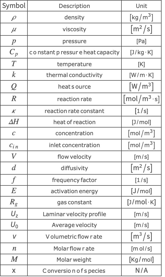
Plot[{temperatureCoupled[r, 0], temperatureCoupled[r, L], temperatureCoupled[r, 0.5 * L]}, {r, 0, Subscript[r, tube]}, ...]Plot[{Subscript[functionx, A][r, 0], Subscript[functionx, A][r, L], Subscript[functionx, A][r, 0.5 * L]}, {r, 0, Subscript[r, tube]}, ...]Nomenclature
References
1. Fogler, H.S. Elements of Chemical Reaction Engineering, 5th ed., Prentice-Hall Inc., New Jersey. (2016).