FindFit[data,expr,pars,vars]
finds numerical values of the parameters pars that make expr give a best fit to data as a function of vars.
FindFit[data,{expr,cons},pars,vars]
finds a best fit subject to the parameter constraints cons.
FindFit[data,exprspec,pars,vars,"prop"]
specifies what fit property prop should be returned.


FindFit
FindFit[data,expr,pars,vars]
finds numerical values of the parameters pars that make expr give a best fit to data as a function of vars.
FindFit[data,{expr,cons},pars,vars]
finds a best fit subject to the parameter constraints cons.
FindFit[data,exprspec,pars,vars,"prop"]
specifies what fit property prop should be returned.
Details and Options


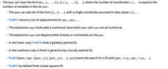
- The data can have the form {{x1,y1,…,f1},{x2,y2,…,f2},…}, where the number of coordinates x, y, … is equal to the number of variables in the list vars.
- The data can also be of the form {f1,f2,…}, with a single coordinate assumed to take values 1, 2, ….
- FindFit returns a list of replacements for par1, par2, ….
- The expression expr must yield a numerical value when pars and vars are all numerical.
- The expression expr can depend either linearly or nonlinearly on the pari.
- The constraints cons can contain equations, inequalities, or logical combinations of these.
- In the linear case, FindFit finds a globally optimal fit.
- In the nonlinear case, it finds in general only a locally optimal fit.
- FindFit[data,expr,{{par1,p1},{par2,p2},…},vars] starts the search for a fit with {par1->p1,par2->p2,…}.
- FindFit by default finds a least‐squares fit.
- The possible fit properties "prop" include:
-
"BestFit" 
the best fit linear combination of basis functions "BestFitParameters" 
the vector  that gives the best fit
"Coordinates" {{x1,y1,…},…} the coordinates of vars in data "FitResiduals" 
the differences between the model and the fit at the coordinates "Function" Function[{x,y,…},a1 f1+…+an fn] best fit pure function "PredictedResponse" 
fitted values for the data coordinates "Response" 
the response vector  from the input data
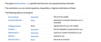
{"prop1","prop2",…} several fit properties - The option NormFunction->f specifies that the norm f[residual] should be minimized.
- The following options can be given:
-
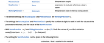
AccuracyGoal Automatic the accuracy sought EvaluationMonitor None expression to evaluate whenever expr is evaluated FitRegularization None regularization for pars for models Gradient Automatic the list of gradient components for expr MaxIterations Automatic maximum number of iterations to use Method Automatic method to use NormFunction Norm the norm to minimize PrecisionGoal Automatic the precision sought StepMonitor None expression to evaluate whenever a step is taken WorkingPrecision Automatic the precision used in internal computations - The default settings for AccuracyGoal and PrecisionGoal are WorkingPrecision/2.
- The settings for AccuracyGoal and PrecisionGoal specify the number of digits to seek in both the values of the parameters returned, and the value of the NormFunction.
- With NormFunction->f and FitRegularization->rfun, Fit finds the values of pars that minimize normf[{expr(pars,x1,y1,…)-f1,…}]+rfun[pars].
- The setting for NormFunction can be given in the following forms:
-
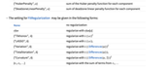
f a function f that is applied to the residual {"HuberPenalty",α} sum of the Huber penalty function for each component {"DeadzoneLinearPenalty",α} sum of deadzone linear penalty function for each component - The setting for FitRegularization may be given in the following forms:
-
None no regularization rfun regularize with rfun[a] {"Tikhonov", λ} regularize with 
{"LASSO",λ} regularize with 
{"Variation",λ} regularize with ![lambda||TemplateBox[{Differences, paclet:ref/Differences}, RefLink, BaseStyle -> {2ColumnTableMod}][a]||^2 lambda||TemplateBox[{Differences, paclet:ref/Differences}, RefLink, BaseStyle -> {2ColumnTableMod}][a]||^2](Files/FindFit.en/11.png)
{"TotalVariation",λ} regularize with ![lambda||TemplateBox[{Differences, paclet:ref/Differences}, RefLink, BaseStyle -> {2ColumnTableMod}][a]||_1 lambda||TemplateBox[{Differences, paclet:ref/Differences}, RefLink, BaseStyle -> {2ColumnTableMod}][a]||_1](Files/FindFit.en/12.png)
{"Curvature",λ} regularize with ![lambda||TemplateBox[{Differences, paclet:ref/Differences}, RefLink, BaseStyle -> {2ColumnTableMod}][a,2]||^2 lambda||TemplateBox[{Differences, paclet:ref/Differences}, RefLink, BaseStyle -> {2ColumnTableMod}][a,2]||^2](Files/FindFit.en/13.png)
{r1,r2,…} regularize with the sum of terms from r1,… - FindFit continues until either of the goals specified by AccuracyGoal or PrecisionGoal is achieved.
- Possible settings for Method include "ConjugateGradient", "PrincipalAxis", "LevenbergMarquardt", "Newton", "NMinimize", and "QuasiNewton", with the default being Automatic.
Examples
open all close allBasic Examples (1)
Scope (7)
Simple Exponential Fitting (3)
Fit data to a model of exponential decay:
Separate the time from the response:
Looking at residuals gives a good indication of whether the model is a good fit:
Use a linear fit on the logarithm of the data for a model of exponential decay:
The logarithm of the exponential model is a linear model for the logarithm of the data:
The exponential model formed by exponentiating the model for the logarithm:
Exponential fit as parameters in a differential equation:
The model function is the solution of a differential equation:
Constraints and Starting Values (2)
Fit to the model with positive amplitude and frequency between 1 and 2:
Compare the fitted model to the data:
The residuals show a pattern, indicating that the frequency constraint is too strict:
Give starting values for some parameters to get a better fit:
Search with all parameters starting at 1:
Options (7)
Gradient (1)
Specify the model gradient to avoid problems with a removable singularity:
With symbolic derivatives FindFit fails since the derivative for Sinc is given as a generic formula:
The gradient has a singularity when ![]() since there is a point in the data with
since there is a point in the data with ![]() :
:
Specify finite differences to avoid the removable singularity:
MaxIterations (1)
When convergence is slow, increasing MaxIterations may allow convergence to the best fit:
With the default, convergence is not reached:
Method (1)
StepMonitor (1)
WorkingPrecision (1)
Use a higher WorkingPrecision to get a more precise parameter estimate:
Applications (7)
Mathematical Data (2)
Experimental Data (3)
Determine the approximate complexity of a computation:
Fit to the theoretical model for the complexity of an FFT:
Show the timing data and the fit in a log-log plot:
Fit a model for lubricant viscosity to experimental data:
Model for lubricant viscosity as a function of temperature ![]() and pressure/1000
and pressure/1000 ![]() :
:
Scale the pressure to improve the conditioning of the model:
Find the parameters ![]() that best fit the scaled data:
that best fit the scaled data:
Show a plot of the fit with the scaled experimental data:
Fit a model for the rate of isomerization of n-pentane to isopentane with experimental data:
Nonlinear model for rate as a function of hydrogen ![]() , n-pentane
, n-pentane ![]() , and isopentane
, and isopentane ![]() :
:
Find the parameters ![]() that best fit the data starting with values having the right size:
that best fit the data starting with values having the right size:
Differential Equations (2)
Find parameters in a differential equation model that give the best fit:
Define a model so the solution for a set of parameters ![]() is reused for all
is reused for all ![]() values:
values:
Find the fit with tolerance appropriate to the precision of the solutions of the ODE:
Show the fitted model with the data and the residuals:
Find how a nonsoliton initial condition for the KdV equation breaks down into two solitons:
The initial wave breaks into two separate waves:
Get the spatial grid used by NDSolve to solve the PDE:
The discretized solution at the final time:
Model of two solitons with different velocities:
Find fit with starting conditions estimated from the graph of the discretized solution:
Plots of the two-soliton model and residuals at intermediate times:
Properties & Relations (6)
FindFit gives the parameter estimates:
NonlinearModelFit allows for extraction of additional information about the fitting:
Extract the parameter estimates:
Extract additional results and diagnostics:
For linear models, Fit and FindFit are equivalent and use LeastSquares:
Use Fit with the basis {1,x,x2}:
This is equivalent to FindFit with the model function a linear combination of the basis:
Construct a design matrix and use LeastSquares to find the coefficients:
LinearModelFit fits linear models and gives additional results about the fitting:
FindFit effectively uses FindMinimum to minimize a norm of the residual function:
The residual is the difference between response and model prediction:
FindFit gives a result consistent with normally distributed responses by default:
LogitModelFit assumes binomially distributed responses:
The same is true for ProbitModelFit:
GeneralizedLinearModelFit allows for binomial and other distributional structures.
Model gamma-distributed responses:
Compare with the result for normally distributed responses:
FindFit will use the time stamps of a TimeSeries as variables:
Rescale the time stamps and fit again:
FindFit acts pathwise on a multipath TemporalData:
See Also
FindMinimum Fit FindFormula NMinimize LeastSquares Interpolation FindCurvePath ChiSquareDistribution LinearModelFit NonlinearModelFit
Function Repository: TrigFit
Related Guides
-
▪
- Curve Fitting & Approximate Functions ▪
- Time Series Processing ▪
- Data Transforms and Smoothing ▪
- Matrix-Based Minimization ▪
- Supervised Machine Learning ▪
- Optimization ▪
- Scientific Data Analysis ▪
- Numerical Data ▪
- Machine Learning ▪
- Signal Visualization & Analysis ▪
- Image Computation for Microscopy
History
Introduced in 2003 (5.0) | Updated in 2007 (6.0) ▪ 2019 (12.0) ▪ 2025 (14.2)
Text
Wolfram Research (2003), FindFit, Wolfram Language function, https://reference.wolfram.com/language/ref/FindFit.html (updated 2025).
CMS
Wolfram Language. 2003. "FindFit." Wolfram Language & System Documentation Center. Wolfram Research. Last Modified 2025. https://reference.wolfram.com/language/ref/FindFit.html.
APA
Wolfram Language. (2003). FindFit. Wolfram Language & System Documentation Center. Retrieved from https://reference.wolfram.com/language/ref/FindFit.html
BibTeX
@misc{reference.wolfram_2025_findfit, author="Wolfram Research", title="{FindFit}", year="2025", howpublished="\url{https://reference.wolfram.com/language/ref/FindFit.html}", note=[Accessed: 09-May-2026]}
BibLaTeX
@online{reference.wolfram_2025_findfit, organization={Wolfram Research}, title={FindFit}, year={2025}, url={https://reference.wolfram.com/language/ref/FindFit.html}, note=[Accessed: 09-May-2026]}