



MovingMap
詳細
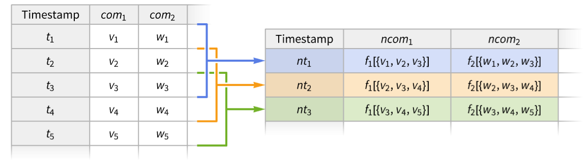
- MovingMapは,ローリングマップまたはスライディングマップとしても知られている.
- MovingMapは,通常,各時間窓の値のリストに関数を適用することによって時系列データを平滑化するために使用される.
- 時系列データ tes の取り得る形式には次のものが含まれる.
-
TimeSeries[…] 連続した時間順に並んだサンプルデータ EventSeries[…] 値を伴う時間的事象の集合 TemporalData[…] 時間と値のペアから構成される1つ以上の経路 {{t1,x1},{t2,x2},…} 時間と値のペアのリスト {x1,x2,…} 0から始まる整数時が暗黙に対応付けられた値のリスト - 1引数の関数 f が,各窓の値のリスト{xi,xi+1,…}に適用される. »
- 純関数 f は,次の引数を使って,各窓についての値,時,境界値,境界時間にアクセスすることができる. »
-
#Values または #1 窓内のデータ値 #Times または #2 窓内のデータ時点 #BoundaryValues または #3 窓の境界でリサンプルされた値 #BoundaryTimes または #4 窓の境界の時点 #Dates または #5 窓内のデータの日付 - デフォルトで,f は各窓について1つの値を計算し,時点は自動的に計算されると期待される.出力を規則{τi,…}{vi,…}として与える関数 f を使うと,時点と値を制御するとともに,1つの窓について複数の値を作成することができる. »
- 可能な窓指定 wspec には次のものが含まれる.
-
size, {size} サイズを指定する(配置および位置は Automatic とする) {size,align} サイズおよび配置を指定する(位置は Automatic とする) {size,align,wpos} サイズ,配置および位置を指定する » - 窓 size は次のように与えることができる.
-
w 日数を意味する正の数 Quantity[w,timeunit] 期間 w (単位:timeunit) Quantity[n,"Events"] n 個の事象数が窓サイズを定義する - "Month"や"Events"のような相対単位を参照する場合,窓サイズは絶対的な意味においては変動し得る.
- 窓のパラメータ{τ1,…,τm} は wpos に特有である.タイムスタンプが{t1,…,tn}のとき,wpos は,次のいずれかである.
-
Automatic data タイムスタンプ τi=tiを使う {τmin,τmax} τmin≤tk+i≤τmaxとなるような τi=tk+iを使う {Automatic,τmax} {t1,τmax}に等しい {τmin,Automatic} {τmin,tn}に等しい {τmin,τmax,dτ} τ1=τmin,τ2=τmin+dτ 等を使う {{τ1,…,τm}} 明示的な τ1,τ2等を使う - デフォルトで,出力のタイムスタンプは窓配置{τ1,…,τm}である.
- 窓の並べ方 align は,窓内の τiの相対位置を決定する.使用可能な設定値には,Right(デフォルト),Left,Centerがある.
- padding の設定値
-
Automatic オーバーハングしない窓だけを保存する(デフォルト) None 充填はせず,すべての窓を保存する valuepadding {Automatic,valuepadding}に等しい {timepadding,valuepadding} 時点と値の充填設定 - valuepadding の設定値は,ArrayPadが認識する任意の有効な指定でよい.
- timepadding の設定
-
Automatic 時点 - 刻み幅の中央値ので一様に Δt 刻み幅 Δt で一様に {Δt1,Δt2,…} ステップ Δtiで循環的に充填 "ReflectedDifferences" 時点間の差の反映 "PeriodicDifferences" ステップ ti+1-tiで循環的に充填 - MovingMapは,複数の経路があるTemporalDataオブジェクトについては,経路ごとに縫い込まれる.


例題
すべて開く すべて閉じる例 (4)
MovingMap[Mean, TimeSeries[{Subscript[x, 1], Subscript[x, 2], Subscript[x, 3], Subscript[x, 4], Subscript[x, 5]}], 2]等間隔に配置された時系列に対しては,各窓は3つの要素の平均を生成する:
Normal[%]ts = TimeSeries[{Subscript[x, 1], Subscript[x, 2], Subscript[x, 3], Subscript[x, 4], Subscript[x, 5], Subscript[x, 6], Subscript[x, 7]}, {Prime[Range[7]]}]Normal[ts]MovingMap[Mean, ts, 3]Normal[%]ts = TimeSeries[TimeEventSeries`TimestampData[Association["UniformlySpacedQ" -> False,
"Timestamps" -> TabularColumn[Association[
"Data" -> {502, {{{1704153600000, 1704240000000, 1704326400000, 1704412800000, 1704672000000,
1704758 ... 0999755859375,
273.3999938964844, 273.760009765625, 273.0799865722656, 271.8599853515625}, {
}, None}}, None}, "ElementType" -> TypeSpecifier["Quantity"]["Real64",
"USDollars"]]]}}]]]], Association[]];ColumnTypes[ts]MovingMap[Mean[#close]&, ts, {Quantity[3, "Months"], Center}]Show[DateListLogPlot[ts -> "close", PlotStyle -> GrayLevel[.7]], DateListLogPlot[%, Joined -> True, PlotStyle -> Thick]]ts = TimeSeries[Accumulate[RandomReal[{-1, 1}, 50]]]MovingMap[{"min" -> (Min[#Values]&), "max" -> (Max[#Values]&)}, ts, {5, Center}]ListLinePlot[{ts, % -> "min", % -> "max"}]スコープ (35)
基本的な用法 (7)
data = {{1, Subscript[x, 1]}, {2, Subscript[x, 2]}, {4, Subscript[x, 4]}, {6, Subscript[x, 6]}, {7, Subscript[x, 7]}, {12, Subscript[x, 12]}};MovingMap[f, data, 2]MovingMap[f, data, Quantity[3, "Events"]]ts = TimeSeries[TimeEventSeries`TimestampData[Association["UniformlySpacedQ" -> True, "Count" -> 6,
"Endpoints" -> TabularColumn[Association["Data" -> {{0, 0}, {}, DataStructure["BitVector",
{"Data" -> ByteArray["/Q=="], "Capacity" -> 2, " ... ne}, "ElementType" ->
"String"]]}}]]]], Association["ResamplingMethod" ->
Association["c1" -> {"Interpolation", InterpolationOrder -> 1}, "c2" -> "PreviousElement"],
"TimeWindow" -> Interval[{0, 5}], "MetaInformation" -> None]];Normal[ts]MovingMap[StringJoin[#c2]&, ts, 2]Normal[%]data = RandomFunction[WienerProcess[], {0, 10, 0.1}]mq = MovingMap[Quantile[#, 0.75]&, data, {1, Center}]ListLinePlot[{data, mq}]data = TimeSeries[Accumulate[RandomReal[{-1, 1}, 250]], {1}]q = MovingMap[Quartiles, data, {12, Center}]ListLinePlot[q]data = TimeSeries[FinancialData["SBUX", {"2020", "2025"}]]RegularlySampledQ[data]MovingMap[Median, data, Quantity[3, "Months"]]Show[DateListLogPlot[data, PlotStyle -> GrayLevel[.7]], DateListLogPlot[%, Joined -> True, PlotStyle -> Thick]]ts = FinancialData["SP500", {"2020", "2025"}]MovingMap[Mean, ts, "Year"]MovingMap[Mean, ts, {"Year", Right, "Month"}]MovingMap[Mean, ts, {"Year", Right, {"Jan 1 2020", Automatic, "Month"}}, "Reflected"]DateListPlot[{ts, %}, Joined -> {False, True}, PlotStyle -> {PointSize[Tiny], Automatic, Automatic}]data = RandomFunction[BrownianBridgeProcess[{0, -1}, {2, 1}], {0, 2, .01}, 3]avg = MovingMap[Mean, data, {0.1, Center}, "Reflected"]Show[ListPlot[data], ListLinePlot[avg]]データの型 (7)
v = Table[Subscript[x, t], {t, 1, 12}]MovingMap[f, v, 2]data = {{"2005", 1}, {"2006", -1}, {"2007", 3}, {"2008", 6}, {"2009", -2}, {"2010", 4}, {"2011", 5}, {"2012", 4}, {"2013", 6}, {"2014", 3}};mavg = MovingMap[Mean, data, "Year"];DateListPlot[{data, mavg}, Joined -> True]TimeSeriesについての移動GeometricMeanを計算する:
ts = TimeSeries[TimeEventSeries`TimestampData[Association["UniformlySpacedQ" -> True, "Count" -> 64,
   "Endpoints" -> TabularColumn[Association["Data" -> {{1, 64}, {}, None},
      "ElementType" -> "Integer64"]], "MinimumTimeIncrement" -> 1, "Caller" ... 87661, 0.2380279869779624, 0.18426497446026752,
      0.13307598834536247, 0.09329283514730177}, {}, None}, "ElementType" -> "Real64"]],
 Association["ResamplingMethod" -> "LinearInterpolation", "TimeObservationWindow" ->
Interval[{1, 64}]]];MovingMap[GeometricMean, ts, 5, None]ListLinePlot[{ts, %}]TemporalDataについての移動中央値を計算する:
td = RandomFunction[ARMAProcess[{5 / 6}, {1 / 2}, 1], {0, 100}]MovingMap[Median, td, 10, None]ListLinePlot[{td, %}]EventSeriesについての移動合計を計算する:
es = EventSeries[TimeEventSeries`TimestampData[Association["UniformlySpacedQ" -> True, "Count" -> 100,
   "Endpoints" -> TabularColumn[Association["Data" -> {{0, 99}, {}, None},
      "ElementType" -> "Integer64"]], "MinimumTimeIncrement" -> 1, "Calle ... , 1, 0, 0, 0, 1, 1, 1, 0, 0, 0, 0, 0, 0, 1, 1, 0, 1, 0, 0, 1, 0, 1, 0, 1, 1, 1,
      0, 0, 1, 1, 1, 0, 0, 1, 1, 1, 1, 1, 0, 0, 0, 1, 1, 0}, {}, None},
"ElementType" -> "Integer64"]], Association["TimeObservationWindow" -> Interval[{0, 99}]]];MovingMap[Total, es, 10]ListPlot[{%, es}, Filling -> 2 -> Axis, Joined -> {True, False}, InterpolationOrder -> 0]td = RandomFunction[BrownianBridgeProcess[], {0, 1, .01}, 3]MovingMap[Variance, td, 0.15]ListLinePlot[%, PlotRange -> All]α = {{.2, .1}, {-.3, .2}};
Σ = {{1, 0.3}, {0.3, .3}};
ar = RandomFunction[ARProcess[{α}, Σ], {1, 5000}]corFunc = Apply[Correlation, Transpose[#]]&;
MovingMap[corFunc, ar, 100]ListLinePlot[%]関数 (7)
data = {{0.2, Subscript[x, 1]}, {0.5, Subscript[x, 2]}, {0.7, Subscript[x, 3]}, {1, Subscript[x, 4]}, {1.1, Subscript[x, 5]}, {1.3, Subscript[x, 6]}};MovingMap[f, data, 0.6]MovingMap[f[#1]&, data, 0.6]MovingMap[f[#Values]&, data, 0.6]data = {{2, Subscript[x, 1]}, {5, Subscript[x, 2]}, {7, Subscript[x, 3]}, {10, Subscript[x, 4]}, {11, Subscript[x, 5]}, {13, Subscript[x, 6]}};MovingMap[f[#1, #2]&, data, 6]MovingMap[f[#Values, #Times]&, data, 6]境界時間と境界時間におけるリサンプルされた値を持つ関数も与える:
MovingMap[f[#Values, #Times, #BoundaryTimes, #BoundaryValues]&, data, 6]//Normalf[vals_, bt_, q_] := {q First[bt] + (1 - q)Last[bt]} -> {Mean[vals]}これを使って,事実上,窓の平均と窓内のスケールされた時点を関連させる:
ts = TimeSeries[Accumulate[RandomReal[{-1, 1}, 21]], {0, Automatic, 0.1}]Table[MovingMap[f[#Values, #BoundaryTimes, q]&, ts, .5], {q, {0, 1 / 4, 1 / 2, 3 / 4, 1}}]//ListLinePlotf[vals_, tms_] := With[{ord = Position[vals, _ ? OddQ]}, Delete[tms, ord] -> Delete[vals, ord]]ts = TimeSeries[RandomVariate[BinomialDistribution[10, .3], 20]]GroupBy[ts["Values"], OddQ]MovingMap[f[#1, #2]&, ts, Quantity[1, "Events"]]Normal[%]es = EventSeries[Range[1990, 2010, 1], {Table[WolframAlpha["thanksgiving date " ~~ ToString[y], {{"Result", 1}, "ComputableData"}], {y, 1990, 2010}]}]MovingMap[DateDifference@@(#Dates)&, es, Quantity[2, "Events"]];DateListPlot[%, Joined -> False, Filling -> Axis]ts = TimeSeries[TimeEventSeries`TimestampData[Association["UniformlySpacedQ" -> True, "Count" -> 61,
"Endpoints" -> TabularColumn[Association[
"Data" -> {2, {{{1756684800000, 1761868800000}, {}, None}}, None},
"ElementType" -> TypeSpeci ... , {}, None}, "ElementType" -> "Integer64"]],
Association["ResamplingMethod" -> "PreviousElement", "TimeObservationWindow" ->
DateInterval[{{{2025, 9, 1, 0, 0, 0.}, {2025, 10, 31, 0, 0, 0.}}}, "Day", "Gregorian", None,
"UT", Automatic]]];DateListPlot[ts]MovingMap[{"minimum" -> (Min[#Values]&), "maximum" -> (Max[#Values]&)}, ts, {Quantity[7, "Days"], Right}]DateListPlot[% -> {"minimum", "maximum"}]es = EventSeries[«3»];ColumnKeys[es]res = MovingMap[Length[#Type]&, es, {Quantity[12, "SynodicMonths"], Right}];Histogram[res]MinMax[res]窓の大きさ (4)
ts = TimeSeries[{Subscript[x, 1], Subscript[x, 2], Subscript[x, 3], Subscript[x, 4], Subscript[x, 5], Subscript[x, 6], Subscript[x, 7], Subscript[x, 8], Subscript[x, 9]}, {1}]MovingMap[f, ts, 2]//Normaldata = FinancialData["APP", "2010"]mvar = MovingMap[GeometricMean, data, Quantity[2, "Quarters"]]DateListPlot[{data, mvar}, Joined -> True]windowSize = {1, "Day"};
winter = WeatherData["Chicago", "Temperature", {"Dec 2024", "Feb 2025"}];MovingMap[Median, winter, {windowSize, Right, {4, "Hour"}}]DateListPlot[%, FrameLabel -> Automatic, GridLines -> {Automatic, Quartiles[winter]}, TargetUnits -> QuantityUnit[winter["FirstValue"]]]es = EventSeries[Table[1, {52}], {RandomSample[DayRange["Jan 1 2025", "Dec 31 2025"], 52]}]windowSize = Quantity[n = 3, "Events"];
eventsPerWeek[times_] := UnitConvert[n / (Last[times] - First[times]), "Weeks" ^ (-1)];MovingMap[eventsPerWeek[#Times]&, es, windowSize]DateListPlot[%, PlotRange -> All, TargetUnits -> (1 / "Weeks"), FrameLabel -> Automatic]窓揃え (4)
data = TimeSeries[{Subscript[x, 1], Subscript[x, 2], Subscript[x, 3], Subscript[x, 4], Subscript[x, 5]}, {1}];MovingMap[f, data, {2, Right}]//NormalMovingMap[f, data, {2}]//Normaldata = TimeSeries[{Subscript[x, 1], Subscript[x, 2], Subscript[x, 3], Subscript[x, 4], Subscript[x, 5]}, {1}];MovingMap[f, data, {2, Center}]//Normaldata = TimeSeries[{Subscript[x, 1], Subscript[x, 2], Subscript[x, 3], Subscript[x, 4], Subscript[x, 5]}, {1}];MovingMap[f, data, {2, Left}]//Normaldata = RandomFunction[PoissonProcess[1.5], {0, 20}]MovingMap[Mean, data, {5, #}]& /@ {Right, Center, Left};Show[ListPlot[data, PlotStyle -> Gray], ListLinePlot[%, PlotStyle -> Thick, PlotLegends -> {Right, Center, Left}]]窓の置き方 (3)
MovingMap[f, Table[{t, Subscript[x, t]}, {t, 9}], {3, Right, Automatic}]MovingMap[f, Table[{t, Subscript[x, t]}, {t, 9}], {3, Right, {5, 8}}]MovingMap[f, Table[{t, Subscript[x, t]}, {t, 9}], {3, Right, {6.5, Automatic}}]path = RandomFunction[PoissonProcess[$VersionNumber], {0, 25}]MovingMap[Last, path, {2, Right, 1}, "Fixed"]MovingMap[Last, path, {2, Right, {0.5, 24.5, 1}}, "Fixed"]cat = FinancialData["CAT", {"2019", "2024"}]pos = Sort@RandomSample[DateRange[cat["FirstDate"], cat["LastDate"]], 100];関心のある各日付について,過去2四半期内の最高株価を求める:
MovingMap[Max, cat, {{2, "Quarter"}, Right, {pos}}];ListLinePlot[{cat, %}]充填 (3)
Automatic充填の場合データの時間領域にオーバーハングしない窓だけが使われる:
data = {{0., Subscript[x, 0]}, {0.7, Subscript[x, 1]}, {1.2, Subscript[x, 2]}, {1.5, Subscript[x, 3]}, {1.9, Subscript[x, 5]}, {2.35, Subscript[x, 6]}};mmR = MovingMap[f, data, {0.8, Right}, Automatic]mmL = MovingMap[f, data, {0.8, Left}, Automatic]mmC = MovingMap[f, data, {0.8, Center}, Automatic]デフォルトではAutomatic充填が使われる:
MovingMap[f, data, 1.7, Automatic]MovingMap[f, data, 1.7]充填をNoneに設定すると,データの時間領域が重なり合う窓が出る:
data = {{0., Subscript[x, 0]}, {0.7, Subscript[x, 1]}, {1.2, Subscript[x, 2]}, {1.5, Subscript[x, 3]}, {1.9, Subscript[x, 5]}, {2.35, Subscript[x, 6]}};mmR = MovingMap[f, data, {0.8, Right, {0.2, 1.7, .5}}, None]Automaticの時間充填と一定の値の充填を使う:
MovingMap[f[#1, #2]&, {{0., Subscript[x, 0]}, {0.7, Subscript[x, 1]}, {1.2, Subscript[x, 2]}, {1.5, Subscript[x, 3]}, {1.9, Subscript[x, 5]}, {2.35, Subscript[x, 6]}}, {1, Right}, {Automatic, p}]アプリケーション (11)
平滑化データと間伐データ (1)
イリノイ州サボイにおけるバレンタインデー付近の解像度が約1分の気温の記録:
temp = WeatherData["KCMI", "Temperature", {DateObject[{2024, 2, 10}, "Day"], DateObject[{2024, 2, 18}, "Day"]}]DateListPlot[temp]TransformMissing[temp, "Interpolation"]ma = MovingMap[Mean[#Values]&, %, {Quantity[1, "Hours"], Right, Quantity[40, "Minutes"]}]DateListPlot[{temp, ma}]市場のボラティリティ (1)
data = FinancialData["SP500", All]MovingMap[StandardDeviation, data, {5 * 365, "Day"}];DateListPlot[%, Joined -> True, PlotStyle -> Thick]MovingMap[InterquartileRange, data, "Year"];DateListPlot[%, Joined -> True, PlotRange -> All]MovingMap[Max[#] - Min[#]&, data, {2, "Year"}];DateListPlot[%, Joined -> True, PlotRange -> All]加重移動平均 (3)
最近の値により重みを置いて,規則的な時系列の移動平均を計算する:
data = TimeSeries[1 + Accumulate@RandomReal[{-1, 1}, 100]];r = 10;wm = MovingMap[Mean[WeightedData[#, Range[r]]]&, data, Quantity[r, "Events"]];ListPlot[{data, wm}, Joined -> {False, True}]wmP = MovingMap[Mean[WeightedData[#, Range[r, 1, -1]]]&, data, Quantity[r, "Events"]];ListPlot[{data, wm, wmP}, Joined -> {False, True, True}, PlotLegends -> {None, "Recent", "Past"}, PlotStyle -> {Brown, Automatic, Automatic}, PlotTheme -> "Detailed"]data = TimeSeries[Accumulate[RandomReal[{-1, 1}, 250]], {1}];wFun[bw_] := Table[HeavisideLambda[(x/#)], {x, -#, #}]&[(bw - 1/2)]ListPlot[wFun[11], Filling -> Axis]w = Range[5, 75, 15];wm = Table[MovingMap[Mean[WeightedData[#, wFun[Length[#]]]]&, data, {bw, Center}, "Reflected"], {bw, w}];Show[ListPlot[data], ListLinePlot[wm, PlotLegends -> w]]ts = TimeSeries[Table[{t, EllipticTheta[1, t, 0.3]}, {t, Join[{0.}, RandomReal[{0, 2Pi}, 254], {2.Pi}]}]]timesToWeights[times_ ? VectorQ] := ListConvolve[{1, 1}, Differences[ArrayPad[times, {1, 1}, "Fixed"]]]区間{t1,tn}内の{{t1,v1},…,{tn,vn}}の線形補間の時間平均:
timeMean[vals_, tms_] := Dot[vals, Normalize[timesToWeights[tms], Total]]mm = MovingMap[timeMean[#Values, #Times]&, ts, {1.6, Right, {0., 2Pi, 0.1}}]int0[s_Real] := NIntegrate[EllipticTheta[1, t, 0.3], {t, s - 1.6, s}] / 1.6Show[Plot[int0[s], {s, mm["FirstTime"], mm["LastTime"]}, PlotStyle -> Orange], ListPlot[mm, Filling -> Axis]]粒子軌道 (2)
n[] := RandomReal[CauchyDistribution[0, 1]]f[] := {u Cos[u] + n[], u Sin[u] + n[]};data = Table[f[], {u, 0, 6π, 1 / 100}];もとになっている信号とノイズを含むシミュレーションによる経路:
{ParametricPlot[{u Cos[u], u Sin[u]}, {u, 0, 6π}], pd = ListPlot[data, AspectRatio -> 1]}移動TrimmedMeanを使って軌道を平滑化する:
td = TimeSeries[data, {0., 6π}, ValueDimensions -> 2];smooth[r_] := MovingMap[TrimmedMean, td, {r, Center}, "Reflected"]Table[ParametricPlot[Evaluate[smooth[r][t]], {t, 0, 6π}], {r, {.15, .25, .50, 1}}]n[] := RandomReal[{-1, 1}]path = TimeSeries[Table[{Sin[u] + n[], Cos[u] + n[], u + n[]}, {u, 0, 6Pi, .1}], Automatic]ParametricPlot3D[path[t], {t, 0, 1885}, BoxRatios -> 1, PlotStyle -> Thin]smooth = MovingMap[Mean, path, {10, Center}]ParametricPlot3D[Normal[smooth[t]], {t, 0, 1885}, BoxRatios -> 1]GARCH過程およびARMA過程 (1)
GARCH(一般化された条件付き分散不均一自己回帰)過程とARMA(自己回帰移動平均)過程のボラティリティを比較する:
g = GARCHProcess[.8, {.6}, {.2}];a = ARMAProcess[{.6}, {.2}, 2];Mean /@ {g[t], a[t]}Variance /@ {g[t], a[t]}garch = RandomFunction[g, {0, 10 ^ 4}];
arma = RandomFunction[a, {0, 10 ^ 4}];GARCH過程については,ボラティリティは特徴的な峰を示す:
mvG = MovingMap[Variance, garch, 100];
mvA = MovingMap[Variance, arma, 100];ListLinePlot[{mvG, mvA}, PlotRange -> All, PlotLegends -> {"GARCH", "ARMA"}]フィルタリング (2)
イリノイ州サボイにおける,バレンタインデー付近のマルチ解像度の気温の記録:
temps = TimeSeries[«3»];maxTempFuncSpec = Function[{v, t}, Module[{ord = Take[Ordering[v], -1]}, t[[ord]] -> v[[ord]]]];minTempFuncSpec = Function[{v, t}, Module[{ord = Take[Ordering[v], 1]}, t[[ord]] -> v[[ord]]]];wSize = Quantity[1, "Day"];
wAlign = Left;
wPos = {DateObject[{2015, 2, 10}], DateObject[{2015, 2, 17}], Quantity[1, "Day"]};maxTS = MovingMap[maxTempFuncSpec, temps, {wSize, wAlign, wPos}, None]minTS = MovingMap[minTempFuncSpec, temps, {wSize, wAlign, wPos}, None]DateListPlot[{temps, maxTS, minTS}, Joined -> {True, False, False}, Filling -> {2 -> {Axis, ColorData[97, 2]}, 3 -> {Axis, ColorData[97, 3]}}, PlotStyle -> {Automatic, PointSize[Medium], PointSize[Medium]}, GridLinesStyle -> Dotted, GridLines -> {AbsoluteTime /@ DateRange[DayRound[#1, All], DayRound[#2, All, "Previous"], "Day"]&, None}, Axes -> True, PlotLegends -> {"Temperature", "Daily Max", "Daily Min"}, PlotTheme -> "Detailed", ImageSize -> Medium]ts = TimeSeries[TimeEventSeries`TimestampData[Association["UniformlySpacedQ" -> True, "Count" -> 61,
"Endpoints" -> TabularColumn[Association[
"Data" -> {2, {{{1756684800000, 1761868800000}, {}, None}}, None},
"ElementType" -> TypeSpeci ... , {}, None}, "ElementType" -> "Integer64"]],
Association["ResamplingMethod" -> "PreviousElement", "TimeObservationWindow" ->
DateInterval[{{{2025, 9, 1, 0, 0, 0.}, {2025, 10, 31, 0, 0, 0.}}}, "Day", "Gregorian", None,
"UT", Automatic]]];Tabular[ts]res = MovingMap[{"maximum" -> (Max[#Values]&), "minimum" -> (Min[#Values]&), "steps" -> (Last[#BoundaryValues]&)}, ts, {Quantity[7, "Days"], Right}]Tabular[res]DateListPlot[res -> {"minimum", "maximum", "steps"}]時点変更ウィナー過程 (1)
WienerProcessのサンプルからOrnsteinUhlenbeckProcessのサンプルを構築する:
wp = RandomFunction[WienerProcess[], {0, 2, 0.01}, 5];


ouPoint[{w_}, {τ_}, {μ_, σ_, θ_, x0_}] := Module[{t = (1/2θ)Log[1 + 2 θ τ], α = (1 + 2 θ τ)^-1 / 2}, {t} -> {μ + (x0 - μ)α + σ α w}]1つの事象窓上で,ウィナー経路の時点と値のペアをOrnstein–Uhlenbeck経路の時点と値のペアにマップする,移動マップを計算する:
oup = MovingMap[ouPoint[#1, #2, {1, 0.3, 5.3, 2}]&, wp, Quantity[1, "Event"]];経路のシミュレーションを可視化し,過程の平均値関数と比較する:
mf[t_] = Mean[OrnsteinUhlenbeckProcess[1, 0.3, 5.3, 2][t]]Show[Plot[mf[t], {t, 0, oup["MaximumTime"]}, PlotStyle -> {Gray, Thick}], ListPlot[oup]]特性と関係 (7)
ts = TimeSeries[{Subscript[x, 1], Subscript[x, 2], Subscript[x, 3], Subscript[x, 4], Subscript[x, 5]}]MovingMap[Mean, ts, 2]Normal[%]MovingMap[Mean, ts, Quantity[3, "Events"]]Normal[%]単純な時系列引数について,マッピングされた関数における#は値を表す:
simpleTS = TimeSeries[{1.2, 2.7, 3.5, 6.7, 8.4, 9.9}, {11}]MovingMap[f[#]&, simpleTS, 2]//Normal単純な時系列を名前付きの成分"a"を持つ新たな時系列に変換する:
compTS = RenameColumns[simpleTS, "Value" -> "a"]#はTabularオブジェクトを表すようになった:
MovingMap[f[#]&, compTS, 2]//NormalMovingMap[f[#a]&, compTS, 2]//NormalTabularColumn入力は,数値関数を含む多くの関数に使える:
MovingMap[Mean[#a]&, compTS, 2]//Normalその他の関数についてはNormalを使う:
MovingMap[f[Normal[#a]]&, compTS, 2]//Normal規則的なデータ上のMeanのMovingMapはMovingAverageに等しい:
data = {Subscript[x, 1], Subscript[x, 2], Subscript[x, 3], Subscript[x, 4], Subscript[x, 5], Subscript[x, 6]};MovingMap[Mean, data, Quantity[3, "Events"]]MovingAverage[data, 3]% === %%規則的なデータ上のMedianのMovingMapはiMovingMedianに等しい:
data = RandomInteger[{-10, 10}, 10]MovingMap[Median, data, Quantity[3, "Events"]]MovingMedian[data, 3]% === %%MovingMapはListConvolveに関連している:
data = {Subscript[x, 1], Subscript[x, 2], Subscript[x, 3], Subscript[x, 4]};r = 3;MovingMap[f, data, r - 1, a]ListConvolve[ConstantArray[1, r], data, {1, 1}, a, Times, f[{##}]&]MovingMapはListCorrelateに関連している:
data = {Subscript[x, 1], Subscript[x, 2], Subscript[x, 3], Subscript[x, 4]};r = 3;MovingMap[f, data, r - 1, a]ListCorrelate[ConstantArray[1, r], data, {-1, -1}, a, Times, f[{##}]&]data = {Subscript[x, 1], Subscript[x, 2], Subscript[x, 3], Subscript[x, 4], Subscript[x, 5], Subscript[x, 6], Subscript[x, 7]};MovingMap[Last[#] - First[#]&, data, 1]Differencesを使うこともできる:
Differences[data]diff[data_, r_ : 1] := MovingMap[#1.((-1)^#1 + Mod[r, 2] Binomial[r, #1]&)[Range[0, r]]&, data, r]diff[data, 2]Table[diff[data, i] == Differences[data, i], {i, 5}]おもしろい例題 (2)
td = Table[u Cos[u], {u, 0, 16π, 0.1}];ListLinePlot[td]Block[{absMax = -Infinity, absMin = Infinity},
max = MovingMap[(absMax = Max[absMax, Max[#]])&, td, 1];
min = MovingMap[(absMin = Min[absMin, Min[#]])&, td, 1];
]ListLinePlot[{min, td, max}, Filling -> {1 -> {2}}]合衆国憲法中のエントロピーの変化を可視化する.同じ単語が繰り返し使われている場合はエントロピーが低くなる:
constitution = StringSplit[ExampleData[{"Text", "USConstitution"}], Except[WordCharacter]..];ListLinePlot[MovingMap[Entropy, constitution, {200, Center}]]数名が自分の名前と出身州をリストする箇所でエントロピーが高くなる:
constitution[[4501 ;; 4607]]大統領の継承に関する米国憲法修正第25条は,比較的繰り返しが多い:
constitution[[7604 ;; 7611]]SortBy[Tally[constitution[[7604 ;; 8015]]], Last][[-10 ;; ]]テキスト
Wolfram Research (2014), MovingMap, Wolfram言語関数, https://reference.wolfram.com/language/ref/MovingMap.html (2026年に更新).
CMS
Wolfram Language. 2014. "MovingMap." Wolfram Language & System Documentation Center. Wolfram Research. Last Modified 2026. https://reference.wolfram.com/language/ref/MovingMap.html.
APA
Wolfram Language. (2014). MovingMap. Wolfram Language & System Documentation Center. Retrieved from https://reference.wolfram.com/language/ref/MovingMap.html