Power

x^y

の乗を与える．

詳細

記号操作・数値操作の両方に適した数学関数である．
の形式の解に，可能な限り，厳密な有理数の結果が与えられる．
複素数とについてPowerは，の主値を与える． »
は，が整数の場合に限って自動的にに変換される．
は，が整数の場合に限って自動的にに変換される．
特別な引数の場合，Powerは自動的に厳密値を計算する．
Powerは任意の数値精度で評価できる．
Powerは自動的にリストに縫い込まれる．
Power[x,y]は，複素平面のから0の範囲において非整数について不連続な分枝切断線を持つ．
Power[x,y,z,…]はPower[x,Power[y,z,…]]と解釈される．
PowerはIntervalオブジェクトおよびCenteredIntervalオブジェクトに使うことができる． »

予備知識

Powerは，式を与えられた数で累乗する数学関数である．式Power[x,y]は通常短縮形のシンタックス x^y を使って表される，あるいは2Dタイプセット形式で x^y として書かれる．ある数の1乗は，それ自体に等しく()，1の複素ベキは1に等しい()．ベキ関数の逆関数は，Logで与えられるので，をについて解くと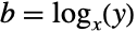，の主要解が返される．
式を2乗する操作は,「平方」として,式の3乗は「立方」として知られる．ベキを含む数量を組み合せる規則は，指数規則と呼ばれ，与えられたベキに底を累乗することは，累乗法として知られる．Power，Exp，Log，およびその関連関数を含む多くの式は，自動的に簡約されるか，SimplifyまたはFullSimplifyを使って簡約される．PowerExpandを使って形式的展開および関連の簡約化を行い，ExpToTrigを使ってPower式の三角法形式を得ることができる．
関数Sqrt[x]は，Power[x,1/2]を使って表される．自然対数の底Eを使った累乗法は，Exp[x]として入力されるが，Power[E,x]を使って表される．
Power[x,y]は，非整数 y についての複素 x 平面でから0まで変化する y の分岐線法の非連続性を持つ．この分岐線法のため，Power[x,1/n]はデフォルトで負の実数 x と奇数の正の数 n について，実数根の代りに複素根を返す．実数値の n 乗根を得るためには，Surd[x,n]を使う．特殊形CubeRoot[x]は，Surd[x,3]に対応する．

例題

すべて開くすべて閉じる

例 (6)

数値的に評価する：

Wolfram Language code: 2 ^ 100

を使って上付き文字として入力する：

Wolfram Language code: 2^100

明示的なFullForm：

Wolfram Language code: Power[2, 100]

実数の部分集合上でプロットする：

Wolfram Language code: Plot[Power[x, 3], {x, 0, 5}]

複素数の部分集合上でプロットする：

Wolfram Language code: ComplexPlot3D[z^3, {z, -3 - 3I, 3 + 3I}, PlotLegends -> Automatic]

特異点における漸近展開：

Wolfram Language code: Series[Power[x^2 / 3], {x, -1, 3}, Assumptions -> Im[x] > 0]

スコープ (46)

数値評価 (9)

数値的に評価する：

Wolfram Language code: Power[2., -1 / 2]

高精度で評価する：

Wolfram Language code: N[((12/17))^5, 50]

結果の最初の百万桁を効率的に計算する：

Wolfram Language code: res = N[Power[123, 4567890], 10 ^ 6];//Timing

必要な場合は複素数が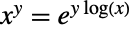生成される：

Wolfram Language code: (-5)^1 / 2

主根は常に使われる：

Wolfram Language code: (-1)^1 / 3

Wolfram Language code: N[%]

これは，として定義されたPowerの一般定義に基づいている：

Wolfram Language code: %% == Exp[(1/3) Log[-1]]

Surdを使って実根を得ることができる：

Wolfram Language code: Surd[-1, 3]

複素数入力：

Wolfram Language code: N[Power[2, I]]

Wolfram Language code: Power[I, 2]

Wolfram Language code: Power[2, I, 2]

Powerは要素単位でリストと行列に縫い込まれる：

Wolfram Language code: {0, 1.5, I π, ∞}^1 / 2

Wolfram Language code: 2 ^ {1, 2, 3}

Wolfram Language code:

(⁠|   |    |
| :- | :- |
| 1 | u  |
| v | I  |⁠)^2//MatrixForm

PowerはIntervalオブジェクトおよびCenteredIntervalオブジェクトに使うことができる：

Wolfram Language code: Interval[{1 / 3, 2}] ^ 3

Wolfram Language code: Pi ^ Interval[{2, 3.}]

Wolfram Language code: CenteredInterval[2, 1 / 100] ^ CenteredInterval[3, 1 / 100]

Wolfram Language code: CenteredInterval[2 + 3I, (1 + I) / 100] ^ CenteredInterval[3, (1 + I) / 100]

Aroundを使って平均的な場合の統計区間を計算する：

Wolfram Language code: Power[ 2, Around[2 / 3, 0.001]]

配列の要素ごとの値を計算する：

Wolfram Language code: Power[2, {{1 / 2, -1}, {-5 / 3, 1 / 2}}]

MatrixFunctionを使って行列のPower関数を計算することもできる：

Wolfram Language code: MatrixFunction[Power[2, #]&, {{1 / 2, -1}, {-5 / 3, 1 / 2}}]//FullSimplify

特定の値 (4)

ゼロにおける値：

Wolfram Language code: Power[x, 0]

Wolfram Language code: Power[0, n]

結果はの実部に応じて0または無限大になる：

Wolfram Language code: {0^2, 0^-2}//Quiet

したがって，以下は不定である：

Wolfram Language code: Power[0, 0]//Quiet

無限大における極限値：

Wolfram Language code: Limit[x ^ n, n -> ∞, Assumptions -> Abs[x] < 1]

Wolfram Language code: Limit[x ^ n, n -> ∞, Assumptions -> Abs[x] > 1]

記号的に評価する：

Wolfram Language code: Power[2, y]

Wolfram Language code: Power[x, 5]

Wolfram Language code: Power[x, y, z]

Power[x,3]=0.5であるような x の値を求める：

Wolfram Language code: xval = x /. FindRoot[Power[x, 3] == 0.5, {x, 0.1}]

結果を可視化する：

Wolfram Language code: Plot[Power[x, 3], {x, 0, 1}, Epilog -> Style[Point[{xval, Power[xval, 3]}], PointSize[Large], Red]]

可視化 (5)

関数を，いくつかの整数 n について実数上でプロットする：

Wolfram Language code: Plot[{x^1, x^2, x^3, x^4}, {x, -1, 1}, PlotLegends -> "Expressions"]

の実部と虚部を実数上でプロットする：

Wolfram Language code: ReImPlot[x^2 / 3, {x, -4, 4}, PlotLegends -> Automatic]

(Power[x,])と (CubeRoot[x]) の実部と虚部を実数上で比較する：

Wolfram Language code: ReImPlot[{x^(1/(3)), Surd[x, 3]}, {x, -4, 4}, PlotLegends -> Automatic]

の実部をプロットする：

Wolfram Language code: ComplexContourPlot[Re[(z)^5 / 2], {z, -3 - 3 I, 3 + 3I}, Contours -> 20]

の虚部をプロットする：

Wolfram Language code: ComplexContourPlot[Im[(z)^5 / 2], {z, -3 - 3 I, 3 + 3I}, Contours -> 20]

を使った極プロット：

Wolfram Language code: PolarPlot[ϕ^3, {ϕ, 0, 8π}, Frame -> True]

関数の特性 (11)

は，のすべての実数について定義される：

Wolfram Language code: FunctionDomain[2^n, n]

のときは，整数についてしか定義されない：

Wolfram Language code: FunctionDomain[(-2)^n, n]

非零のについては，の整関数である：

Wolfram Language code: FunctionDomain[(-2)^n, n, Complexes]

の関数範囲：

Wolfram Language code: FunctionRange[2^n, n, y]

Wolfram Language code: FunctionRange[2^n, n, z, Complexes]

Powerは右結合である：

Wolfram Language code: Power[x, y, z] === Power[x, Power[y, z]]

右辺の形式が望ましい形である：

Wolfram Language code: Power[x, y, z]//FullForm

Powerは，複素平面上で第2引数において周期的である：

Wolfram Language code: FunctionPeriod[x ^ n, n, Complexes]

分岐における極限を求める：

Wolfram Language code: Limit[(-2 + ε) ^ (1 / 3), ε -> 0, Direction -> I]

Wolfram Language code: Limit[(-2 + ε) ^ (1 / 3), ε -> 0, Direction -> -I]

Wolfram Language code: N[{%, %%}]

固定の正の整数については，はの解析関数である：

Wolfram Language code: FunctionAnalytic[x^n, x, Assumptions -> n∈ℤ && n > 0]

負の整数については解析的ではないが有理型ではある：

Wolfram Language code: FunctionMeromorphic[x^n, x, Assumptions -> n∈ℤ && n < 0]

非整数については，有理型でさえない：

Wolfram Language code: {FunctionMeromorphic[x^1 / 2, x], FunctionMeromorphic[x^-π, x]}

固定の非零の実数については，はの解析関数である：

Wolfram Language code: FunctionAnalytic[b^x, x, Assumptions -> b∈ℝ && b ≠ 0]

2変数関数としては，は解析的でも有理型でもない：

Wolfram Language code: {FunctionAnalytic[x^y, {x, y}], FunctionMeromorphic[x^y, {x, y}]}

はについては増加する：

Wolfram Language code: FunctionMonotonicity[b^x, x, Assumptions -> b > 1, StrictInequalities -> True]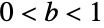

については減少する：

Wolfram Language code: FunctionMonotonicity[b^x, x, Assumptions -> 0 < b < 1, StrictInequalities -> True]

は，についてを除いては単射である：

Wolfram Language code: FunctionInjective[b^x, x, Assumptions -> b < -1 || b > 1 || -1 < b < 0 || 1 > b > 0]

について可視化する：

Wolfram Language code: Plot[{((1/4))^``x``, 5}, {x, -5, 5}]

はの任意の値について実数への全射ではない：

Wolfram Language code: FunctionSurjective[b^x, x, Assumptions -> b > 1]

について可視化する：

Wolfram Language code: Plot[{4^``x``, -2}, {x, -5, 5}]

はについて正である：

Wolfram Language code: FunctionSign[b^``x``, x, Assumptions -> b > 0, StrictInequalities -> True]

は偶数のについて非負である：

Wolfram Language code: FunctionSign[x^n, x, Assumptions -> (n/2)∈ℤ && n > 0]

はまたはについて一般的な特異点を持つ：

Wolfram Language code: FunctionSingularities[x^n, x]

しかし，についてで連続的である：

Wolfram Language code: FunctionContinuous[{x ^ n, x ≥ 0}, x]//FullSimplify

はについて凸である：

Wolfram Language code: FunctionConvexity[b^x, x, Assumptions -> b > 0]

は正の偶数について凸である：

Wolfram Language code: FunctionConvexity[x^n, x, Assumptions -> (n/2)∈ℤ && n > 0]

微分 (4)

x についての一次導関数：

Wolfram Language code: D[Power[x, n], x]

x についての高次導関数：

Wolfram Language code: Table[D[Power[x, n], {x, k}], {k, 1, 4}]//FullSimplify

高次導関数を x についてプロットする：

Wolfram Language code:

Plot[Evaluate[% /. n -> 4], {x, -3, 3}, PlotLegends -> {"First Derivative", "Second Derivative", "Third Derivative", "Fourth Derivative"}]

x についての次導関数の式：

Wolfram Language code: D[Power[x, n], {x, k}]// FullSimplify

第2引数についての導関数：

Wolfram Language code: D[x^n, n]

次導関数：

Wolfram Language code: D[x^n, {n, k}]

積分 (3)

Integrateを使って不定積分を計算する：

Wolfram Language code: Integrate[x^y, x]// FullSimplify

不定積分を確かめる：

Wolfram Language code: FullSimplify[D[%, x]]// FullSimplify

定積分：

Wolfram Language code: Integrate[x^y, {x, 0, 10}, Assumptions -> Re[y] > -1]

その他の積分例：

Wolfram Language code: Integrate[x^y y^x, x]// FullSimplify

Wolfram Language code: Integrate[Log10[x] Power[E, x], {x, 0, E}]// FullSimplify

級数展開 (4)

Seriesを使ってテイラー(Taylor)展開を求める：

Wolfram Language code: Series[Power[y, x], {x, 0, 5}]

の周りの最初の3つの近似をプロットする：

Wolfram Language code:

terms = Normal@Table[Series[Power[2, x], {x, 0, m}], {m, 1, 5, 2}];
Plot[{Power[2, x], terms}, {x, -10, 10}]

SeriesCoefficientを使った級数展開の一般項：

Wolfram Language code: SeriesCoefficient[Power[y, x], {x, 1, n}]

一次フーリエ(Fourier)級数：

Wolfram Language code: FourierSeries[Power[y, x], x, 1]// FullSimplify

生成点におけるテイラー展開：

Wolfram Language code: Series[Power[y, x], {x, x0, 2}]// FullSimplify

関数の恒等式と簡約 (6)

主定義：

Wolfram Language code: Power[z, 0] == 1

Wolfram Language code: Power[z, k] == z Power[z, k - 1]

オイラーの公式：

Wolfram Language code: ExpToTrig[Power[E, I x]]

Exp関数との結合：

Wolfram Language code: Power[-1, a] == Exp[I a π]//FullSimplify

ネストしたベキは常に自動的に結合されるわけではない：

Wolfram Language code: (x ^ 2)^1 / 3

PowerExpandを使って強制的に簡約する：

Wolfram Language code: PowerExpand[%]

以下は不正な結果を生成することがある：

Wolfram Language code: (x ^ 2)^1 / 3 == PowerExpand[x^2 / 3] /. x -> -1

あるいは，Simplifyで適切な仮定を使う：

Wolfram Language code: Simplify[(x ^ 2)^1 / 3, x∈Reals]

積は自動的に繋がれる：

Wolfram Language code: Power[x, a]Power[x, b]

実変数 x および y を仮定して展開する：

Wolfram Language code: ComplexExpand[Power[x + I y, k]]

アプリケーション (5)

5%複利：

Wolfram Language code: Table[(1 + 0.05) ^ n, {n, 5}]

側の立方体と同じ体積の球の半径を求める：

Wolfram Language code: Reduce[(4/3)Pi r ^ 3 == a ^ 3, r, Reals]

Wolfram Language code: ToRadicals[%, Assumptions -> a > 0]

Wolfram Language code: % /. a -> 1.

複素逆ベキの等高線プロット：

Wolfram Language code: ContourPlot[Re[2 ^ (1 / (0.1 + x + I y))], {x, -0.1, 0.1}, {y, -0.1, 0.1}]

有理関数の積分をLogについて求める：

Wolfram Language code: Integrate[1 / (x ^ 2 - 1), x]

有理係数がある変数を持つ微分方程式を解く：

Wolfram Language code: DSolve[{(1 + x^2) y''[x] + 2 x y'[x] == 0, y[0] == 0, y'[0] == 1}, y[x], x]

特性と関係 (27)

平方根の等価形式：

Wolfram Language code: {x ^ (1 / 2), Sqrt[x], Sqrt[x]}

根のベキは全体的に自動的に簡約される：

Wolfram Language code: (z ^ (1 / 3)) ^ 3

ベキの根は自動的には簡約されない：

Wolfram Language code: (z ^ 3) ^ (1 / 3)

Wolfram Language code: (z ^ 3) ^ (1 / 3) /. z -> -1

Power[x,1/n]またはを使って主複素根を求める：

Wolfram Language code: (-16.)^1 / 4

Wolfram Language code: -32.^(1/(5))

Surd[x,n]を使って n 番目の実根を求める：

Wolfram Language code: Surd[-16., 4]

Wolfram Language code: Surd[-32., 5]

仮定をもって簡約する：

Wolfram Language code: Simplify[(z ^ 3) ^ (1 / 3), z > 0]

PowerExpandを使って形式的に簡約する：

Wolfram Language code: PowerExpand[(z ^ 3) ^ (1 / 3)]

すべての複素数に有効な結果を得る：

Wolfram Language code: PowerExpand[(z ^ 3) ^ (1 / 3), Assumptions -> {}]

Wolfram Language code: PiecewiseExpand[%, Assumptions -> -Pi < Arg[z] ≤ Pi]

ExpToTrigを使って三角法の形を求める：

Wolfram Language code: (-1) ^ (1 / 7)

Wolfram Language code: ExpToTrig[(-1) ^ (1 / 7)]

単独の根に簡約する：

Wolfram Language code: RootReduce[2 ^ (1 / 2) + 5 ^ (1 / 5)]

SolveまたはRootを使ってすべての根を求める：

Wolfram Language code: sol = Solve[x ^ 6 == 1, x]

Wolfram Language code: root = Table[Root[# ^ 6 - 1&, m], {m, 6}]

表現形式や順序は異なるが，これらはの根は等しい：

Wolfram Language code: Sort[ExpToTrig[x /. sol]] == Sort[root]

Expandを使って多項式のベキに展開する：

Wolfram Language code: (1 + x) ^ 10

Wolfram Language code: Expand[(1 + x) ^ 10]

ベキは自動的に級数に適用される：

Wolfram Language code: Series[Exp[x], {x, 0, 5}]

Wolfram Language code: % ^ 4

ベキを含む方程式には無限に多くの解があることがある：

Wolfram Language code: Solve[a ^ x == b, x]

Wolfram Language code: Reduce[a ^ x == b, x]//TraditionalForm

逆数や平方根等は自動的にベキに変換される：

Wolfram Language code: 1 / x ^ 2//FullForm

Wolfram Language code: Sqrt[x]//FullForm

指数関数はベキに変換される：

Wolfram Language code: Exp[x] // FullForm

のベキをマッチする：

Wolfram Language code: Cases[{1 / x, 1, Sqrt[x], x, x ^ 2, x ^ 3}, x ^ _]

の場合を含む：

Wolfram Language code: Cases[{1 / x, 1, Sqrt[x], x, x ^ 2, x ^ 3}, x ^ _.]

複素平面上の分数ベキの分枝切断線構造：

Wolfram Language code: Plot3D[Im[(x + I y) ^ (1 / 3)], {x, -3, 3}, {y, -2, 2}]

ベキが代数的かどうかテストする：

Wolfram Language code: (2 + Sqrt[3]) ^ (1 / 3)∈Algebraics

Wolfram Language code: (Pi) ^ (1 / 3)∈Algebraics

積分：

Wolfram Language code: ∫x^aa^xⅆx

積分変換：

Wolfram Language code: LaplaceTransform[t^n, t, s]

Wolfram Language code: FourierTransform[1 / t ^ 2, t, s]

総和：

Wolfram Language code: Underoverscript[∑, k = Subscript[k, 1], Subscript[k, 2]]k^a

微分方程式：

Wolfram Language code: DSolve[z Derivative[1][w][z] - a w[z] == 0, w[z], z]

Powerは多くの数学関数の特殊形に現れる：

Wolfram Language code: {HypergeometricPFQ[{-a}, {}, 1 - z], Hypergeometric2F1[-a, b, b, 1 - z], MeijerG[{{1 + a}, {}}, {{0}, {}}, z - 1]}

PowerはDifferenceRootとして表すことができる：

Wolfram Language code: DifferenceRootReduce[Power[k, 2], k]

Wolfram Language code: DifferenceRootReduce[Power[z, k], k]

Powerの級数展開における一般項：

Wolfram Language code: SeriesCoefficient[Power[a, x], {x, 0, n}]

Powerの母関数：

Wolfram Language code: GeneratingFunction[Power[n, k], n, x]

Wolfram Language code: Series[%, {x, 0, 10}]

FindSequenceFunctionはPower数列を認識する：

Wolfram Language code: Table[Power[n, 5], {n, 10}]

Wolfram Language code: FindSequenceFunction[%, n]

Powerの指数母関数：

Wolfram Language code: ExponentialGeneratingFunction[Power[k, n], n, x]

GeneralizedPowerを使って任意の二項演算の整数乗を表す：

Wolfram Language code: GeneralizedPower[NonCommutativeMultiply, x + y, 3]

PowerはTimesのGeneralizedPowerである：

Wolfram Language code: GeneralizedPower[Times, x, k]

考えられる問題 (13)

Powerは常に主根を計算する：

Wolfram Language code: (-1) ^ (1 / 3)

Wolfram Language code: N[%]

ベキは一般的に根の逆ではない：

Wolfram Language code: (z ^ 3) ^ (1 / 3)

Wolfram Language code: (z ^ 3) ^ (1 / 3) /. z -> -1

Wolfram Language code: PowerExpand[(z ^ 3) ^ (1 / 3)]

近似値の場合，虚部が生成される：

Wolfram Language code: ((-1.) ^ (1 / 3)) ^ 3

Wolfram Language code: ((N[-1, 20]) ^ (1 / 3)) ^ 3

Chopを使って小さい虚部を削除する：

Wolfram Language code: Chop[%]

分枝切断線によってこの関数は不連続になる：

Wolfram Language code: Plot[Sqrt[z ^ 2] / z, {z, -1, 1}]

しかし，この導関数は一般的に簡約すると0になる：

Wolfram Language code: D[Sqrt[z ^ 2] / z, z]

機械精度の場合，分枝切断線上で不正確な数値結果が与えることがある：

Wolfram Language code: N[(-2 + I ((Pi + 1) ^ 2 - Pi ^ 2 - 2Pi - 1 - Exp[-Pi ^ 4])) ^ (1 / 3)]

Wolfram Language code: N[(-2 + I ((Pi + 1) ^ 2 - Pi ^ 2 - 2Pi - 1 - Exp[-Pi ^ 4])) ^ (1 / 3), 8]

機械数による入力は任意精度の結果を与えることがある：

Wolfram Language code: 5 ^ 5 ^ 5.

Wolfram Language code: MachineNumberQ[%]

ベキは非常に大きくなることがある：

Wolfram Language code: 2 ^ 2 ^ 20.

ベキの中にはどのようなコンピュータにとっても大きすぎるものもある：

Wolfram Language code: 2 ^ 2 ^ 100.

ベキは不定式を与えることがある：

Wolfram Language code: 0 ^ 0

各結果の精度は零の精度によって決まる：

Wolfram Language code: {x ^ 0, x ^ 0.0, x ^ 0``10}

1の記号ベキは1が厳密数あるいは機械精度数である場合にのみ評価される：

Wolfram Language code: {1 ^ x, 1.0 ^ x, 1``10 ^ x}

デフォルト設定での数値操作ではこのベキは簡約できない：

Wolfram Language code: (Pi ^ 2 + 2Pi + 1 - (Pi + 1) ^ 2 + Exp[-1000]) ^ 0

機械精度数の評価では不十分である：

Wolfram Language code: N[%]

より高い内部精度を使うと結果が結合される：

Wolfram Language code: Block[{$MaxExtraPrecision = 10 ^ 4}, N[%%, 20]]

非有理数のベキは級数に吸収されない：

Wolfram Language code: Series[x ^ Sqrt[2] Sin[x], {x, 0, 5}]

Wolfram Language code: Head[%]

Powerは行列に対して要素単位で適用される：

Wolfram Language code: {{1, 2}, {3, 4}} ^ 2

行列のベキにはMatrixPowerを使う：

Wolfram Language code: MatrixPower[{{1, 2}, {3, 4}}, 2]

おもしろい例題 (3)

連続するベキをプロットする：

Wolfram Language code: Plot[Evaluate[Table[x ^ n, {n, 10}]], {x, -1.2, 1.2}]

連続する指数塔を生成する：

Wolfram Language code: NestList[z ^ #&, z, 6]

そのような塔の引数の等高線プロット：

Wolfram Language code:

ContourPlot[Evaluate[Sin[Arg[z^z^z^z /. z -> x + I y] / 2]], {x, -1, 1}, {y, -1, 1}, ColorFunction -> Hue, ContourStyle -> None, Exclusions -> {}]

の指数塔の大きさ：

Wolfram Language code: ListPlot[Abs[NestList[I ^ #&, 1, 50]]]

極限を求める：

Wolfram Language code: FixedPoint[SetPrecision[I ^ #, 16]&, 1]

極限について解く：

Wolfram Language code: Solve[I ^ x == x, x]

Wolfram Language code: N[%, 16]

Top

その他のラーニングリソース

テクニカルサポート

データサイエンス，金融，ビジネス

工学

科学とテクノロジー

教育のためのテクノロジー

教育イニシアチブ

使い始める

Grow Your Skills

Wolframと繋がる

大人用の教育プログラム

若者のための教育プログラム

読む

Power

詳細

予備知識

例題

例 (6)

スコープ (46)

数値評価 (9)

特定の値 (4)

可視化 (5)

関数の特性 (11)

微分 (4)

積分 (3)

級数展開 (4)

関数の恒等式と簡約 (6)

アプリケーション (5)

特性と関係 (27)

考えられる問題 (13)

おもしろい例題 (3)

テキスト

CMS

APA

BibTeX

BibLaTeX

Power

詳細

予備知識

例題

例 (6)

スコープ (46)

数値評価 (9)

特定の値 (4)

可視化 (5)

関数の特性 (11)

微分 (4)

積分 (3)

級数展開 (4)

関数の恒等式と簡約 (6)

アプリケーション (5)

特性と関係 (27)

考えられる問題 (13)

おもしろい例題 (3)

関連項目

テクニカルノート

関連するガイド

関連リンク

履歴

テキスト

CMS

APA

BibTeX

BibLaTeX