

AcousticPDEComponent
AcousticPDEComponent[vars,pars]
yields an acoustic PDE term component with variables vars and parameters pars.
Details
- AcousticPDEComponent returns a sum of differential operators to be used as a part of partial differential equations:
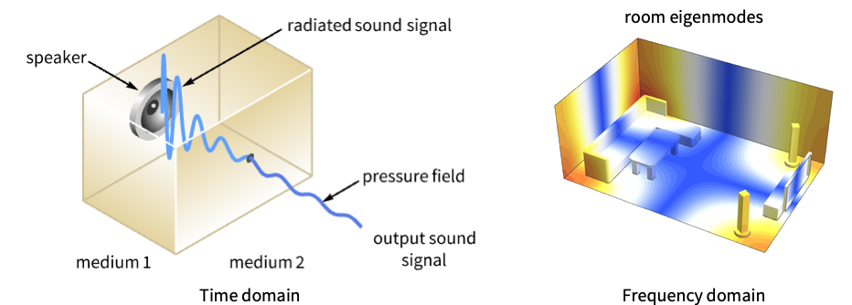
- AcousticPDEComponent models the propagation of sound in isotropic media in both the time and frequency domain by mechanisms such as diffusion.
- AcousticPDEComponent models acoustic phenomena in fluids with dependent variable pressure
 [
[![TemplateBox[{InterpretationBox[, 1], "Pa", pascals, "Pascals"}, QuantityTF]](Files/AcousticPDEComponent.en/4.png "TemplateBox[{InterpretationBox[, 1], \"Pa\", pascals, \"Pascals\"}, QuantityTF]") ], independent variables
], independent variables  [
[![TemplateBox[{InterpretationBox[, 1], "m", meters, "Meters"}, QuantityTF]](Files/AcousticPDEComponent.en/6.png "TemplateBox[{InterpretationBox[, 1], \"m\", meters, \"Meters\"}, QuantityTF]") ] and time variable
] and time variable  [
[![TemplateBox[{InterpretationBox[, 1], "s", seconds, "Seconds"}, QuantityTF]](Files/AcousticPDEComponent.en/8.png "TemplateBox[{InterpretationBox[, 1], \"s\", seconds, \"Seconds\"}, QuantityTF]") ] or frequency variable
] or frequency variable  [
[![TemplateBox[{InterpretationBox[, 1], {"rad", , "/", , "s"}, radians per second, {{(, "Radians", )}, /, {(, "Seconds", )}}}, QuantityTF]](Files/AcousticPDEComponent.en/10.png "TemplateBox[{InterpretationBox[, 1], {\"rad\", , \"/\", , \"s\"}, radians per second, {{(, \"Radians\", )}, /, {(, \"Seconds\", )}}}, QuantityTF]") ].
]. - Time-dependent variables vars are vars={p[t,x1,…,xn],t,{x1,…,xn}}.
- Frequency-dependent variables vars are vars={p[x1,…,xn],ω,{x1,…,xn}}.
- The time domain acoustics model AcousticPDEComponent is based on a wave equation with time variable
 , density
  , sound speed
  and sound sources
  and
and  :
: - The frequency domain acoustics model AcousticPDEComponent is based on a Helmholtz equation with angular frequency
 :
: - The units of the acoustic PDE terms are in units of [1/
![TemplateBox[{InterpretationBox[, 1], {{"s", ^, 2}}, seconds squared, {"Seconds", ^, 2}}, QuantityTF]](Files/AcousticPDEComponent.en/19.png "TemplateBox[{InterpretationBox[, 1], {{\"s\", ^, 2}}, seconds squared, {\"Seconds\", ^, 2}}, QuantityTF]") ].
]. - The following parameters pars can be given:
-
parameter default symbol "DipoleSource" {0,…}  , dipole source [
![TemplateBox[{InterpretationBox[, 1], {"N", , "/", , {"m", ^, 3}}, newtons per meter cubed, {{(, "Newtons", )}, /, {(, {"Meters", ^, 3}, )}}}, QuantityTF]](Files/AcousticPDEComponent.en/21.png "TemplateBox[{InterpretationBox[, 1], {\"N\", , \"/\", , {\"m\", ^, 3}}, newtons per meter cubed, {{(, \"Newtons\", )}, /, {(, {\"Meters\", ^, 3}, )}}}, QuantityTF]") ]
]"MassDensity" 1  , density of media [
![TemplateBox[{InterpretationBox[, 1], {"kg", , "/", , {"m", ^, 3}}, kilograms per meter cubed, {{(, "Kilograms", )}, /, {(, {"Meters", ^, 3}, )}}}, QuantityTF]](Files/AcousticPDEComponent.en/23.png "TemplateBox[{InterpretationBox[, 1], {\"kg\", , \"/\", , {\"m\", ^, 3}}, kilograms per meter cubed, {{(, \"Kilograms\", )}, /, {(, {\"Meters\", ^, 3}, )}}}, QuantityTF]") ]
]"Material" Automatic 
"MonopoleSource" 0  , monopole source [1/
![TemplateBox[{InterpretationBox[, 1], {{"s", ^, 2}}, seconds squared, {"Seconds", ^, 2}}, QuantityTF]](Files/AcousticPDEComponent.en/26.png "TemplateBox[{InterpretationBox[, 1], {{\"s\", ^, 2}}, seconds squared, {\"Seconds\", ^, 2}}, QuantityTF]") ]
]"RegionSymmetry" None 
"SoundSpeed" 1  , speed of sound [
![TemplateBox[{InterpretationBox[, 1], {"m", , "/", , "s"}, meters per second, {{(, "Meters", )}, /, {(, "Seconds", )}}}, QuantityTF]](Files/AcousticPDEComponent.en/29.png "TemplateBox[{InterpretationBox[, 1], {\"m\", , \"/\", , \"s\"}, meters per second, {{(, \"Meters\", )}, /, {(, \"Seconds\", )}}}, QuantityTF]") ]
] - All parameters may depend on any of
 ,
,  and
and  as well as other dependent variables with the exception of
  , resulting in a nonlinear eigenvalue problem.
 - AcousticPDEComponent allows for sources in the time domain and sources in the frequency domain.
-
Monopole source, 
Wolfram Language code: [image]Dipole source, 
Wolfram Language code: [image] - A monopole source
 models a point source that radiates sound isotropically.
 - A dipole source
 models a two-point source that radiates sound anisotropically.
 - The number of independent variables in
 specifies the length of
  .
. - If no parameters are specified, the default time domain acoustics PDE is
- If no parameters are specified, the default frequency domain acoustics PDE is
- A possible choice for the parameter "RegionSymmetry" is "Axisymmetric".
- "Axisymmetric" region symmetry represents a truncated cylindrical coordinate system where the cylindrical coordinates are reduced by removing the angle variable as follows:
-
dimension reduction equation 1D 

2D 

- If the AcousticPDEComponent depends on parameters
 that are specified in the association pars as …,keypi…,pivi,…, the parameters
  are replaced with
  .
.
Examples
open all close allBasic Examples (4)
Define a time domain acoustic PDE term:
AcousticPDEComponent[{p[t, x], t, {x}}, <||>]Define a frequency domain acoustic model:
AcousticPDEComponent[{p[x], ω, {x}}, <||>]Define model variables vars for a transient acoustic pressure field with model parameters pars:
vars = {p[t, x], t, {x}};
pars = <|"SoundSpeed" -> 343, "MassDensity" -> 1.2|>;
Define initial conditions ics of a right-going sound wave ![]() :
:
p0 = D[0.125 Erf[(x - 0.5) / 0.15], x];
ics = {p[0, x] == p0, Derivative[1, 0][p][0, x] == -343 * D[p0, x]};
Set up the equation with a sound hard boundary at the right end:
eqn = AcousticPDEComponent[vars, pars] == AcousticSoundHardValue[x == 1, vars, pars]pfun = NDSolveValue[{eqn, ics}, p, {t, 0, 0.003}, x∈Line[{{0}, {1}}]];Visualize the sound field in the time domain:
Manipulate[Plot[pfun[t, x], {x, 0, 1}, ...], {{t, 0}, 0, 0.003, 10 ^ -4}, Rule[...]]Define model variables vars for a frequency domain acoustic pressure field with model parameters pars:
vars = {p[x], ω, {x}};
pars = <|"SoundSpeed" -> 343, "MassDensity" -> 1.2|>;
Set up the equation with a radiation boundary at the left end:
eqn = AcousticPDEComponent[vars, pars] == AcousticRadiationValue[x == 0, vars, pars, <|"SoundIncidentPressure" -> 1|>];pfun = ParametricNDSolveValue[eqn, p, x∈Line[{{0}, {1}}], {ω}];Visualize the sound field in the frequency domain at various frequencies ![]() :
:
Plot[Table[Legended[Abs[pfun[ω][x]], ω], {ω, {1000π, 1500π, 2000π}}]//Evaluate, {x, 0, 1}, ...]Scope (21)
Basic Uses (2)
Time Domain (7)
Define model variables vars for a transient acoustic pressure field with model parameters pars:
vars = {p[t, x], t, {x}};
pars = <|"SoundSpeed" -> 343, "MassDensity" -> 1.2|>;
Set up initial conditions ics of a right-going plane wave ![]() :
:
p0 = D[0.125 Erf[(x - 0.5) / 0.15], x];
ics = {p[0, x] == p0, Derivative[1, 0][p][0, x] == -343 * D[p0, x]};
Set up the equation with an acoustic absorbing boundary at the right end for a plane wave:
eqn = AcousticPDEComponent[vars, pars] == AcousticAbsorbingValue[x == 1, vars, pars];pfun = NDSolveValue[{eqn, ics}, p, {t, 0, 0.003}, x∈Line[{{0}, {1}}]];Manipulate[Plot[pfun[t, x], {x, 0, 1}, ...], {{t, 0.0013}, 0, 0.003, 10 ^ -4}, Rule[...]]Define model variables vars for a transient acoustic pressure field with model parameters pars:
vars = {p[t, x], t, {x}};
pars = <|"SoundSpeed" -> 317, "MassDensity" -> 1.41|>;
Define initial conditions ics of a right-going plane wave ![]() :
:
p0 = D[0.125 Erf[(x - 0.5) / 0.15], x];
ics = {p[0, x] == p0, Derivative[1, 0][p][0, x] == -317 * D[p0, x]};
Set up the equation with an acoustic impedance boundary at the right and an impedance ![]() of
of ![]() :
:
eqn = AcousticPDEComponent[vars, pars] == AcousticImpedanceValue[x == 1, vars, <|"SpecificAcousticImpedance" -> 287.33|>];pfun = NDSolveValue[{eqn, ics}, p, {t, 0, 0.003}, x∈Line[{{0}, {1}}]];Manipulate[Plot[pfun[t, x], {x, 0, 1}, ...], {{t, 0.0006}, 0, 0.003, 10 ^ -4}, Rule[...]]Define model variables vars for a transient acoustic pressure field with model parameters pars:
vars = {p[t, x], t, {x}};
pars = <|"SoundSpeed" -> 343, "MassDensity" -> 1.2|>;
Define silent initial conditions ics:
ics = {p[0, x] == 0, Derivative[1, 0][p][0, x] == 0};Set up the equation with an acoustic normal velocity boundary with the sound particle velocity v of ![]() at the left end:
at the left end:
eqn = AcousticPDEComponent[vars, pars] == AcousticNormalVelocityValue[x == 0, vars, pars, <|"AcousticSoundParticleVelocity" -> Sin[800π t]|>];Solve the PDE on a refined mesh:
pfun = NDSolveValue[{eqn, ics}, p, {t, 0, 0.0025}, x∈Line[{{0}, {1}}], Method -> {"PDEDiscretization" -> {"MethodOfLines", "SpatialDiscretization" -> {"FiniteElement", "MeshOptions" -> {"MaxCellMeasure" -> 0.015}}}}];Manipulate[Plot[pfun[t, x], {x, 0, 1}, ...], {{t, 0.0012}, 0, 0.0025, 10 ^ -4}, Rule[...]]Define model variables vars for a transient acoustic pressure field with model parameters pars:
vars = {p[t, x], t, {x}};
pars = <|"SoundSpeed" -> 343, "MassDensity" -> 1.2|>;
Define silent initial conditions ics:
ics = {p[0, x] == 0, Derivative[1, 0][p][0, x] == 0};Set up the equation with an acoustic pressure boundary and a pressure source ![]() of
of ![]() at the left end:
at the left end:
eqn = {AcousticPDEComponent[vars, pars] == 0, AcousticPressureCondition[x == 0, vars, pars, <|"AcousticPressure" -> Sin[800π t]|>]};Solve the PDE on a refined mesh:
pfun = NDSolveValue[{eqn, ics}, p, {t, 0, 0.0025}, x∈Line[{{0}, {1}}], Method -> {"PDEDiscretization" -> {"MethodOfLines", "SpatialDiscretization" -> {"FiniteElement", "MeshOptions" -> {"MaxCellMeasure" -> 0.015}}}}];Manipulate[Plot[pfun[t, x], {x, 0, 1}, ...], {{t, 0.001}, 0, 0.0025, 10 ^ -4}, Rule[...]]Define model variables vars for a frequency domain acoustic pressure field with model parameters pars:
vars = {p[t, x], t, {x}};
pars = <|"SoundSpeed" -> 343, "MassDensity" -> 1.2|>;
Define silent initial conditions ics:
ics = {p[0, x] == 0, Derivative[1, 0][p][0, x] == 0};Set up the equation with an acoustic radiation boundary at the left end, a pressure source ![]() of
of ![]() and a radiation angle
and a radiation angle ![]() of
of ![]() :
:
eqn = AcousticPDEComponent[vars, pars] == AcousticRadiationValue[x == 0, vars, pars, <|"SoundIncidentPressure" -> Sin[800π t]|>];pfun = NDSolveValue[{eqn, ics}, p, {t, 0, 0.01}, x∈Line[{{0}, {1}}]];Manipulate[Plot[pfun[t, x], {x, 0, 1}, ...], {{t, 0.0074}, 0, 0.01, 10 ^ -4}, Rule[...]]Define model variables vars for a transient acoustic pressure field with model parameters pars:
vars = {p[t, x], t, {x}};
pars = <|"SoundSpeed" -> 343, "MassDensity" -> 1.2|>;
Define initial conditions ics of a right-going plane wave ![]() :
:
p0 = D[0.125 Erf[(x - 0.5) / 0.15], x];
ics = {p[0, x] == p0, Derivative[1, 0][p][0, x] == -343 * D[p0, x]};
Set up the equation with an acoustic sound hard boundary at the right end:
eqn = AcousticPDEComponent[vars, pars] == AcousticSoundHardValue[x == 1, vars, pars];pfun = NDSolveValue[{eqn, ics}, p, {t, 0, 0.003}, x∈Line[{{0}, {1}}]];Manipulate[Plot[pfun[t, x], {x, 0, 1}, ...], {{t, 0.0016}, 0, 0.003, 10 ^ -4}, Rule[...]]Define model variables vars for a transient acoustic pressure field with model parameters pars:
vars = {p[t, x], t, {x}};
pars = <|"SoundSpeed" -> 343, "MassDensity" -> 1.2|>;
Define initial conditions ![]() of a right-going plane wave
of a right-going plane wave ![]() :
:
p0 = D[0.125 Erf[(x - 0.5) / 0.15], x];
ics = {p[0, x] == p0, Derivative[1, 0][p][0, x] == -343 * D[p0, x]};
Set up the equation with an acoustic sound soft boundary at the right end:
eqn = {AcousticPDEComponent[vars, pars] == 0, AcousticSoundSoftCondition[x == 1, vars, pars]};pfun = NDSolveValue[{eqn, ics}, p, {t, 0, 0.003}, x∈Line[{{0}, {1}}]];Manipulate[Plot[pfun[t, x], {x, 0, 1}, ...], {{t, 0.0022}, 0, 0.003, 10 ^ -4}, Rule[...]]Frequency Domain (10)
Define a frequency domain acoustic model with particular sound speed and mass density:
AcousticPDEComponent[{p[x], ω, {x}}, <|"SoundSpeed" -> c, "MassDensity" -> ρ|>]Define a frequency domain acoustic model for a particular material:
AcousticPDEComponent[{p[x], ω, {x}}, <|"Material" -> Entity["Element", "Argon"]|>]Define a frequency domain acoustic model for a particular material:
AcousticPDEComponent[{p[x], ω, {x}}, Entity["Element", "Argon"]]Define model variables vars for a frequency domain acoustic pressure field with model parameters pars:
vars = {p[x], ω, {x}};
pars = <|"SoundSpeed" -> 343, "MassDensity" -> 12 / 10|>;
Set up the equation with a radiation boundary at the left end and an acoustic absorbing boundary at the right end:
eqn = AcousticPDEComponent[vars, pars] == AcousticRadiationValue[x == 0, vars, pars, <|"SoundIncidentPressure" -> 1|>] + AcousticAbsorbingValue[x == 1, vars, pars]pfun = ParametricNDSolveValue[eqn, p, x∈Line[{{0}, {1}}], {ω}];Visualize the solution in the frequency domain at various frequencies ![]() :
:
Plot[Table[Legended[Abs[pfun[ω][x]], ω], {ω, {1000π, 1500π, 2000π}}]//Evaluate, {x, 0, 1}, ...]Convert the solution to the time domain:
Plot[Table[Legended[Re[pfun[ω][x] * Exp[I ω t]], ω], {t, {0.01}}, {ω, {1000π, 1500π, 2000π}}]//Evaluate, {x, 0, 1}, ...]Define model variables vars for a frequency domain acoustic pressure field with model parameters pars:
vars = {p[x], ω, {x}};
pars = <|"SoundSpeed" -> 343, "MassDensity" -> 1.2|>;
Set up the equation with a radiation boundary at the left, an acoustic impedance boundary at the right and an impedance ![]() of
of ![]() :
:
eqn = AcousticPDEComponent[vars, pars] == AcousticRadiationValue[x == 0, vars, pars, <|"SoundIncidentPressure" -> 1|>] + AcousticImpedanceValue[x == 1, vars, pars, <|"SpecificAcousticImpedance" -> 200|>];pfun = ParametricNDSolveValue[eqn, p, x∈Line[{{0}, {1}}], {ω}];Visualize the solution in the frequency domain at various frequencies ![]() :
:
Plot[Table[Legended[Abs[pfun[ω][x]], ω], {ω, {1000π, 1500π, 2000π}}]//Evaluate, {x, 0, 1}, ...]Convert the solution to the time domain:
Plot[Table[Legended[Re[pfun[ω][x] * Exp[I ω t]], ω], {t, {0.01}}, {ω, {1000π, 1500π, 2000π}}]//Evaluate, {x, 0, 1}, ...]Define model variables vars for a frequency domain acoustic pressure field with model parameters pars:
vars = {p[x], ω, {x}};
pars = <|"SoundSpeed" -> 343, "MassDensity" -> 1.2|>;
Set up the equation with an acoustic normal velocity boundary at the left, the sound particle velocity ![]() of
of ![]() and an acoustic absorbing boundary at the right:
and an acoustic absorbing boundary at the right:
eqn = AcousticPDEComponent[vars, pars] == AcousticNormalVelocityValue[x == 0, vars, pars, <|"AcousticSoundParticleVelocity" -> 0.01|>] + AcousticAbsorbingValue[x == 1, vars, pars];pfun = ParametricNDSolveValue[eqn, p, x∈Line[{{0}, {1}}], {ω}];Visualize the solution in the frequency domain at various frequencies ![]() :
:
Manipulate[Plot[Abs[pfun[ω][x]], {x, 0, 1}, ...], {{ω, 1000π, "f"}, {1000π, 1500π, 2000π}}, Rule[...]]Convert the solution to the time domain:
Manipulate[Plot[Re[pfun[ω][x] * Exp[I ω t]], {x, 0, 1}, ...], {{t, 0, "t"}, 0, 0.01}, {{ω, 1000π, "f"}, {1000π, 1500π, 2000π}}, Rule[...]]Define model variables vars for a frequency domain acoustic pressure field with model parameters pars:
vars = {p[x], ω, {x}};
pars = <|"SoundSpeed" -> 343, "MassDensity" -> 1.2|>;
Set up the equation with an acoustic pressure boundary at the left, a pressure source ![]() of
of ![]() and an acoustic absorbing boundary at the right:
and an acoustic absorbing boundary at the right:
eqn = AcousticPDEComponent[vars, pars] == AcousticPressureCondition[x == 0, vars, pars, <|"AcousticPressure" -> 1|>] + AcousticAbsorbingValue[x == 1, vars, pars];pfun = ParametricNDSolveValue[eqn, p, x∈Line[{{0}, {1}}], {ω}];Visualize the solution in the frequency domain at various frequencies ![]() :
:
Manipulate[Plot[Abs[pfun[ω][x]], {x, 0, 1}, ...], {{ω, 1000π, "f"}, {1000π, 1500π, 2000π}}, Rule[...]]Convert the solution to the time domain:
Manipulate[Plot[Re[pfun[ω][x] * Exp[I ω t]], {x, 0, 1}, ...], {{t, 0, "t"}, 0, 0.01}, {{ω, 1000π, "f"}, {1000π, 1500π, 2000π}}, Rule[...]]Define model variables vars for a frequency domain acoustic pressure field with model parameters pars:
vars = {p[x], ω, {x}};
pars = <|"SoundSpeed" -> 343, "MassDensity" -> 1.2|>;
Set up the equation with an acoustic radiation boundary at the left end, a pressure source ![]() of
of ![]() and a radiation angle
and a radiation angle ![]() of
of ![]() :
:
eqn = AcousticPDEComponent[vars, pars] == AcousticRadiationValue[x == 0, vars, pars, <|"SoundIncidentPressure" -> 1|>];pfun = ParametricNDSolveValue[eqn, p, x∈Line[{{0}, {1}}], {ω}];Visualize the solution in the frequency domain at various frequencies ![]() :
:
Plot[Table[Legended[Abs[pfun[ω][x]], ω], {ω, {1000π, 1500π, 2000π}}]//Evaluate, {x, 0, 1}, ...]Convert the solution to the time domain:
Plot[Table[Legended[Re[pfun[ω][x] * Exp[I ω t]], ω], {t, {0.01}}, {ω, {1000π, 1500π, 2000π}}]//Evaluate, {x, 0, 1}, ...]Define model variables vars for a frequency domain acoustic pressure field with model parameters pars:
vars = {p[x], ω, {x}};
pars = <|"SoundSpeed" -> 343, "MassDensity" -> 1.2|>;
Set up the equation with an acoustic radiation boundary at the left, a pressure source ![]() of
of ![]() and an acoustic sound hard boundary at the right:
and an acoustic sound hard boundary at the right:
eqn = AcousticPDEComponent[vars, pars] == AcousticSoundHardValue[x == 1, vars, pars] + AcousticRadiationValue[x == 0, vars, pars, <|"SoundIncidentPressure" -> 1|>];pfun = ParametricNDSolveValue[eqn, p, x∈Line[{{0}, {1}}], {ω}];Visualize the solution in the frequency domain at various frequencies ![]() :
:
Plot[Table[Legended[Abs[pfun[ω][x]], ω], {ω, {1000π, 1500π, 2000π}}]//Evaluate, {x, 0, 1}, ...]Convert the solution to the time domain:
Plot[Table[Legended[Re[pfun[ω][x] * Exp[I ω t]], ω], {t, {0.01}}, {ω, {1000π, 1500π, 2000π}}]//Evaluate, {x, 0, 1}, ...]Define model variables vars for a frequency domain acoustic pressure field with model parameters pars:
vars = {p[x], ω, {x}};
pars = <|"SoundSpeed" -> 343, "MassDensity" -> 1.2|>;
Set up the equation with a radiation boundary at the left end and an acoustic absorbing boundary at the right end:
eqn = {AcousticPDEComponent[vars, pars] == AcousticRadiationValue[x == 0, vars, pars, <|"SoundIncidentPressure" -> 1|>], AcousticSoundSoftCondition[x == 1, vars, pars]};pfun = ParametricNDSolveValue[eqn, p, x∈Line[{{0}, {1}}], {ω}];Visualize the solution in the frequency domain at various frequencies ![]() :
:
Plot[Table[Legended[Abs[pfun[ω][x]], ω], {ω, {1000π, 1500π, 2000π}}]//Evaluate, {x, 0, 1}, ...]Convert the solution to the time domain:
Plot[Table[Legended[Re[pfun[ω][x] * Exp[I ω t]], ω], {t, {0.01}}, {ω, {1000π, 1500π, 2000π}}]//Evaluate, {x, 0, 1}, ...]Units (2)
Set up an acoustic time domain equation for xenon:
AcousticPDEComponent[{p[t, x], t, {x}}, <|"Material" -> ["Xe"]|>] == 0Set up an acoustic frequency domain model for xenon by specifying material parameters:
AcousticPDEComponent[{p[x], ω, {x}}, <|"SoundSpeed" -> ["sound speed xenon"], "MassDensity" -> ["Xe"][EntityProperty["Element", "Density"]]|>] == 0Applications (1)
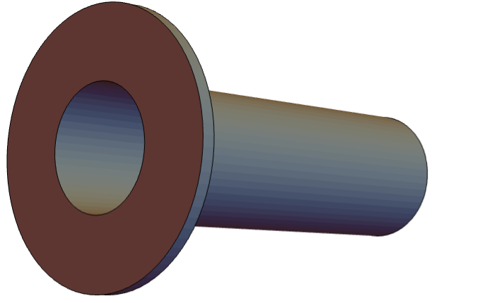
The following acoustic model describes an open pipe, wherein a vibrating piston is placed inside one end of the pipe while the other end of the pipe opens into an infinite domain. In this case, an impedance boundary condition is placed on one end to model the infinite domain. The pipe that will be modeled is a flanged circular pipe, as shown in the following figure:
Since the geometry of the pipe and the boundary conditions are rotationally symmetric about the ![]() axis, an axisymmetric model can be used. The governing equation for describing the sound wave propagation is the axisymmetric Helmholtz equation.
axis, an axisymmetric model can be used. The governing equation for describing the sound wave propagation is the axisymmetric Helmholtz equation.
Set up the variables and parameters:
vars = {p[r, z], ω, {r, z}};
pars  = <|"MassDensity" -> Subscript[ρ, air], "SoundSpeed" -> Subscript[c, air], Subscript[c, air] -> 343, Subscript[ρ, air] -> 1.25, "RegionSymmetry" -> "Axisymmetric"|>;
The axisymmetric geometry can be approximated by a 2D rectangle, which represents a cross-section of the pipe in the ![]() plane:
plane:
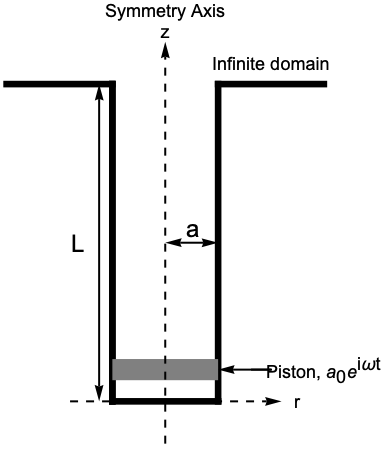
Set up the rectangle region with ![]() as the radius of the tube and
as the radius of the tube and ![]() as the length of the tube:
as the length of the tube:
a = 0.25;
L = 1.5;
Ω = Polygon[{{0, -L}, {a, -L}, {a, 0}, {0, 0}}];
In the model, there are two boundary conditions. One is a NeumannValue, which expresses the acceleration of the piston ![]() with
with ![]() :
:
a0 = 1;
Subscript[Τ, acc] = NeumannValue[a0, z == -L];
The second boundary condition is an AcousticImpedanceValue with impedance ![]() . The impedance
. The impedance ![]() is given by the following approximation, where
is given by the following approximation, where ![]() is the wavenumber:
is the wavenumber:
k = ω / Subscript[c, air];
Subscript[Z, end] = Subscript[ρ, air] * Subscript[c, air] * (1 - (2 BesselJ[1, 2 k a]/2 k a) + I((2 StruveH[1, 2 k a]/2 k a)));
Subscript[Γ, i] = AcousticImpedanceValue[z == 0, vars, pars, <|"SpecificAcousticImpedance" -> Subscript[Z, end]|>];pde = AcousticPDEComponent[vars, pars] == Subscript[Τ, acc] + Subscript[Γ, i];Solve the PDE with ![]() with a MaxCellMeasure defined by
with a MaxCellMeasure defined by ![]() and with a resolution of 12 to get an accurate result:
and with a resolution of 12 to get an accurate result:
λ = 2π Subscript[c, air] / ω;
pfun = ParametricNDSolveValue[pde, p, {r, z}∈Ω, {ω}, Method -> {"PDEDiscretization" -> {"FiniteElement", "MeshOptions" -> {"MaxCellMeasure" -> {"Length" -> λ / 12} /. pars}}}];
pfun1000 = pfun[ω] /. {ω -> (2 Pi)1000};
Visualize the pressure distribution in the full 3D region:
Legended[RegionPlot3D[x^2 + y^2 ≤ a^2 && 0 ≤ PlanarAngle[{0, 0} -> {{a, 0}, {x, y}}] ≤ (4 π/3), {x, -a, a}, {y, -a, a}, {z, -L, 0}, ...], BarLegend[...]]Text
Wolfram Research (2020), AcousticPDEComponent, Wolfram Language function, https://reference.wolfram.com/language/ref/AcousticPDEComponent.html (updated 2023).
CMS
Wolfram Language. 2020. "AcousticPDEComponent." Wolfram Language & System Documentation Center. Wolfram Research. Last Modified 2023. https://reference.wolfram.com/language/ref/AcousticPDEComponent.html.
APA
Wolfram Language. (2020). AcousticPDEComponent. Wolfram Language & System Documentation Center. Retrieved from https://reference.wolfram.com/language/ref/AcousticPDEComponent.html