GibbsPointProcess
GibbsPointProcess[{"PairPotential",μ, ϕ}, d]
represents a Gibbs point process with density μ and pair-potential function ϕ in ![]() .
.
GibbsPointProcess[{"PairInteraction",μ, h}, d]
represents a Gibbs point process with density μ and pair-interaction function h in ![]() .
.
GibbsPointProcess[{"Papangelou",λ*}, d]
represents a Gibbs point process with Papangelou conditional density ![]() in
in ![]() .
.
GibbsPointProcess[{"Density",f}, d]
represents a Gibbs point process with density function proportional to f in ![]() .
.
Details


- GibbsPointProcess is also known as a Markov point process.
- The Gibbs model is typically used to model interaction between points, such as trees or plants competing for resources, or particles repulsing or attracting each other.
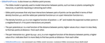
- Gibbs point processes that only have interactions between pairs of points can be specified in terms of their density function
 and the radial pair potential function
  or a pair interaction function
  .
. - The density function
 is a non-negative function of position
  and models the expected number points in a neighborhood of
  if no point interactions are present.
 - The pair potential
 is a real function of the distance between points; higher values of
  mean it is less likely to find two points at distance
  from each other.
 - The pair interaction
 , given by
  , is a non-negative function of the distance between points; a higher value of
  indicates that it is more likely to find two points at distance
  from each other.
 - GibbsPointProcess can represent any Gibbs point process; common Gibbs processes have dedicated implementations and are easier to use:
-
process pair potential 
characteristic HardcorePointProcess 
hardcore interaction StraussPointProcess 
constant strength softcore interaction StraussHardcorePointProcess 
inner hardcore with an outer softcore PenttinenPointProcess 
interaction based on overlapping area DiggleGrattonPointProcess 
inner hardcore with decreasing softcore DiggleGatesPointProcess 
smooth transition from point hardcore - More general Gibbs point processes can be specified in terms of either their Papangelou density
 or probability density
  .
. - The Papangelou density
 specifies the cost of adding a point
  to collection of points
  and needs to be a non-negative function.
 - The density
 specifies the probability density of a point configuration. The function f needs to be non-negative, but not necessarily normalized.
 - GibbsPointProcess allows d to be any positive integer.
- All specifications have an equivalent Papangelou density λ* given by:
-
{"PairPotential",μ,ϕ} ![mu exp(-sum_iphi(TemplateBox[{{{p, _, i}, -, q}}, Norm])) mu exp(-sum_iphi(TemplateBox[{{{p, _, i}, -, q}}, Norm]))](Files/GibbsPointProcess.en/32.png)
{"PairInteraction",μ,h} ![mu product_ip(TemplateBox[{{{p, _, i}, -, q}}, Norm]) mu product_ip(TemplateBox[{{{p, _, i}, -, q}}, Norm])](Files/GibbsPointProcess.en/33.png) .
.{"Density",f} 
- GibbsPointProcess can be used with such functions as RipleyK and RandomPointConfiguration.
Examples
open allclose allBasic Examples (1)
Sample a Poisson point process by GibbsPointProcess with the appropriate density function:
Scope (4)
Simulate a Gibbs point process with density proportional to the number of points:
Use the Markov chain Monte Carlo method to simulate 40 samples over a unit disk:
Compute the average number of points in the region:
Compare to the scaled area of the region:
Sample a Strauss point process by GibbsPointProcess:
Sample the same process by specifying the Papangelou conditional density:
Sample the same process by specifying the pair potential function:
Sample from a hardcore point process with radius 0.3 with respect to a Poisson point process with density ![]() :
:
Compare to the corresponding inhomogeneous Poisson point process simulation:
Simple Gibbs point processes like the StraussHardcorePointProcess have densities that can be expressed solely in terms of the intensity ![]() and pair potential
and pair potential ![]() , but this is not true in general. A point process that depends on the area of the union of disks around the points has interactions that depend on all possible subsets of points, like the density function below demonstrates:
, but this is not true in general. A point process that depends on the area of the union of disks around the points has interactions that depend on all possible subsets of points, like the density function below demonstrates:
Define a Gibbs point process with this density:
Properties & Relations (1)
Compare numbers of points generated with a PoissonPointProcess and a GibbsPointProcess with the appropriate density:
Compute the average number of points in the region for each process simulation:
Text
Wolfram Research (2020), GibbsPointProcess, Wolfram Language function, https://reference.wolfram.com/language/ref/GibbsPointProcess.html.
CMS
Wolfram Language. 2020. "GibbsPointProcess." Wolfram Language & System Documentation Center. Wolfram Research. https://reference.wolfram.com/language/ref/GibbsPointProcess.html.
APA
Wolfram Language. (2020). GibbsPointProcess. Wolfram Language & System Documentation Center. Retrieved from https://reference.wolfram.com/language/ref/GibbsPointProcess.html