

ParametricNDSolveValue
ParametricNDSolveValue[eqns,expr,{x,xmin,xmax},pars]
パラメータが pars,独立変数 x(範囲は xminから xmaxまで)の常微分方程式 eqns の数値解によって決定された関数を使って expr の値を与える.
ParametricNDSolveValue[eqns,expr,{x,xmin,xmax},{y,ymin,ymax},pars]
偏微分方程式 eqns を矩形領域上で解く.
ParametricNDSolveValue[eqns,expr,{x,y}∈Ω,pars]
偏微分方程式 eqns を領域Ω上で解く.
ParametricNDSolveValue[eqns,expr,{t,tmin,tmax},{x,y}∈Ω,pars]
時間依存偏微分方程式 eqns を領域Ω上で解く.
詳細とオプション
- ParametricNDSolveValueは結果をParametricFunctionオブジェクトによって返す.
- {pspec1,pspec2,…}のパラメータ pars の指定を使って範囲を指定することができる.
- pspeciの可能な形式
-
p p は領域RealsまたはComplexesを持つ Element[p,Reals] p は領域Realsを持つ Element[p,Complexes] p は領域Complexesを持つ Element[p,{v1,…}] p は離散範囲{v1,…}を持つ {p,pmin,pmax} p の範囲は 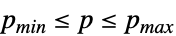 である
- 一般に,expr は微分方程式の解を通してパラメータに間接的に依存しているが,パラメータに明示的に依存していることもある.
- パラメータについての結果のParametricFunctionオブジェクトの導関数は,可能な場合は数値感度メソッドと記号感度メソッドを組み合せて計算される.
- ParametricNDSolveValueにはNDSolveと同じオプションと設定が使える.
- NDSolveとParametricNDSolveValueは,一般に,方程式のタイプによっていくつかの異なる段階に分けて微分方程式を解く.Method->{s1->m1,s2->m2,…}とすると,段階 siがメソッド miで処理される.実際に使われる段階とその順序は,解く問題に基づいてNDSolveによって決定される.
- 可能な解の段階はNDSolveのものに以下を加えたものである.
-
"ParametricCaching" 計算された解をキャッシュする "ParametricSensitivity" パラメータについての導関数の計算
全オプションのリスト
例題
すべて開く すべて閉じる例 (3)
pfun = ParametricNDSolveValue[{y'[t] == a y[t], y[0] == 1}, y, {t, 0, 10}, {a}]y1 = pfun[1]
y1[10]Plot[Evaluate[Table[pfun[a][t], {a, -1, 1, .1}]], {t, 0, 1}, PlotRange -> All]
pfun = ParametricNDSolveValue[{f''[t] + a f[t] == 0, f[0] == 1, f'[0] == 0}, f[10], {t, 0, 10}, {a}]Plot[pfun[a], {a, 0, 2}]関数をFindRootと一緒に使って根を求める:
FindRoot[pfun[a], {a, 1}]pfun = ParametricNDSolveValue[{f''[t] + a f[t] == 0, f[0] == b, f'[0] == 0}, f, {t, 0, 20}, {a, b}];Plot[Evaluate[(pfun[a, b][t] + {0, .1, -.1}D[pfun[a, b][t], a]) /. {a -> 1, b -> 1}], {t, 0, 20}, Filling -> {2 -> {3}}]Plot[Evaluate[(pfun[a, b][t] + {0, .1, -.1}D[pfun[a, b][t], b]) /. {a -> 1, b -> 1}], {t, 0, 20}, Filling -> {2 -> {3}}]スコープ (6)
パラメータ依存性 (4)
ParametricNDSolveValueはParametricFunctionオブジェクトを返す:
pfun = ParametricNDSolveValue[{y''[t] + y[t] == 3a Sin[y[t]], y[0] == y'[0] == 1}, y, {t, 0, 5}, {a}]
if0 = pfun[0]
Plot[if0[t], {t, 0, 5}]


Plot[Evaluate@Table[pfun[a][t], {a, -.5, .5, .05}], {t, 0, 5}, PlotRange -> All]pfun = ParametricNDSolveValue[{y''[t] + 2y[t] == Sin[.4t] + Cos[y[t]], y[0] == a, y'[0] == b}, y, {t, 0, 10}, {a, b}]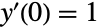


Plot[Evaluate@Table[pfun[a, 1][t], {a, -2, 2, .5}], {t, 0, 10}, PlotRange -> All]


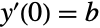
Plot[Evaluate@Table[pfun[1, b][t], {b, -2, 2, .5}], {t, 0, 10}, PlotRange -> All]
eqns = {y''[t] + y[t] == 3a Sin[y[t]], y[0] == y'[0] == 1};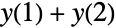
pfun = ParametricNDSolveValue[eqns, y[1] + y[2], {t, 0, 5}, {a}];Plot[pfun[a], {a, -2, 2}]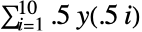
pfun = ParametricNDSolveValue[eqns, Underoverscript[∑, i = 1, 10]0.5 y[0.5 i], {t, 0, 5}, {a}];Plot[pfun[a], {a, -2, 2}]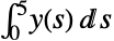
pfun = ParametricNDSolveValue[eqns, Subsuperscript[∫, 0, 5]y[s]ⅆs, {t, 0, 5}, {a}];Plot[pfun[a], {a, -2, 2}]
pfun = ParametricNDSolveValue[eqns, y'[3], {t, 0, 5}, {a}];Plot[pfun[a], {a, -2, 2}]
pfun = ParametricNDSolveValue[eqns, y[a], {t, 0, 5}, {a}];Plot[pfun[a], {a, 0, 5}]pfun = ParametricNDSolveValue[{u''[x] == a u[x], DirichletCondition[u[x] == 1, x == 0], DirichletCondition[u[x] == b, x == 1]}, u, {x}∈Line[{{0}, {1}}], {a, b}] から
 の範囲の
 の値に対して
 で,
 および
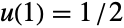 で解をプロットする:
Plot[Evaluate@Table[pfun[a, 1 / 2][t], {a, -2, 2, .5}], {t, 0, 10}, PlotRange -> All]パラメータ感度 (2)
pfun = ParametricNDSolveValue[{y''[t] + y[t] == 0, y[0] == a, y'[0] == 0}, y, {t, 0, 10}, {a}];

Show[Plot[Evaluate@Table[pfun[a][t], {a, 1, 3, .2}], {t, 0, 10}, PlotStyle -> Thin], Plot[pfun[2][t], {t, 0, 10}]] についての
 の感度は定義によると
 である.
 における感度をプロットする:
Plot[pfun'[2][t], {t, 0, 10}]


Plot[Evaluate[pfun[2][t] + {-1, 0, 1}pfun'[2][t]], {t, 0, 10}, PlotStyle -> {Gray, {Blue}, Gray}, Filling -> {1 -> {3}}]pfun = ParametricNDSolveValue[{y''[t] + 2y[t] == Sin[t] + Cos[y[t]], y[0] == a, y'[0] == b}, y, {t, 0, 10}, {a, b}];ifun = pfun[1, 1] および
 における
 という初期条件について感度をプロットする:
ifuna = D[pfun[a, 1], a] /. a -> 1;Plot[Evaluate[ifun[t] + {-.5, 0, .5}ifuna[t]], {t, 0, 10}, PlotStyle -> {Gray, {Blue}, Gray}, Filling -> {1 -> {3}}] および
 における
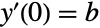 という初期条件について感度をプロットする:
ifunb = D[pfun[1, b], b] /. b -> 1;Plot[Evaluate[ifun[t] + {-.5, 0, .5}ifunb[t]], {t, 0, 10}, PlotStyle -> {Gray, {Blue}, Gray}, Filling -> {1 -> {3}}]一般化と拡張 (2)
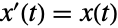 ,
 をさまざまな値のWorkingPrecisionについて解き,誤差をプロットする:
err = ParametricNDSolveValue[{x'[t] == x[t], x[0] == 1}, Abs[x[1] - E], {t, 0, 1}, {wp}, Method -> "Extrapolation", WorkingPrecision -> wp ];ListLogPlot[Table[{wp, err[wp]}, {wp, 16, 60}]]NDSolveValueが直接解けない,高度に非線形な問題の解を求めることを考える.境界条件,領域,パラメータ  に依存する方程式を設定する:
eqn[p_] := Inactive[Div][((x ^ 2 + 3) * D[u[x], x] ^ (p - 1)) Inactive[Grad][u[x], {x}], {x}] - Sin[x]
bc = DirichletCondition[u[x] == 0, True];
Ω = Line[{{0}, {1}}];NDSolveValueは解を求めることができない:
NDSolveValue[{eqn[3] == 0, bc}, u, Element[{x}, Ω]]

Clear[seeding]
seeding[x_ ? NumericQ] := 0
パラメータ  に基づいてParametricNDSolveValue関数を作成する:
psol = ParametricNDSolveValue[{eqn[p] == 0, bc}, u, Element[{x}, Ω], {p}, InitialSeeding -> {u[x] == seeding[x]}]
s1 = psol[1]
Clear[seeding]
seeding[x_ ? NumericQ] := s1[x]
s2 = psol[3]Plot[s2[x], {x, 0, 1}]オプション (2)
Method (2)
ParametricCaching (1)
pfun = ParametricNDSolveValue[{x''[t] + a x[t] == 0, x[0] == b, x'[0] == 0}, x, {t, 0, 1000}, {a, b}, MaxSteps -> ∞, Method -> {"ParametricCaching" -> None}];キャッシュしないと,必要となる唯一の余分なメモリは処理した方程式のためのものになる:
Do[Print[Module[{m = MemoryInUse[]}, AbsoluteTiming[{ByteCount[pfun[2, 2]], MemoryInUse[] - m}]]], {3}]


pfun = ParametricNDSolveValue[{x''[t] + a x[t] == 0, x[0] == b, x'[0] == 0}, x, {t, 0, 1000}, {a, b}, MaxSteps -> ∞];Do[Print[Module[{m = MemoryInUse[]}, AbsoluteTiming[{ByteCount[pfun[2, 2]], MemoryInUse[] - m}]]], {3}]


ParametricSensitivity (1)
pfun = ParametricNDSolveValue[{x'[t] == a x[t], x[0] == b}, x[1], {t, 0, 1}, {a, b}, Method -> {"ParametricSensitivity" -> None}];Plot3D[pfun[a, b], {a, 1, 2}, {b, 0, 1}]dfun = Derivative[1, 0][pfun];
dfun[1, 1]アプリケーション (15)
パラメータスイープ (8)
さまざまな高さから落とされて弾むボールのシミュレーションを行う:
pfun = ParametricNDSolveValue[{y''[t] == -9.8bounce[t], y[0] == height, y'[0] == 0, bounce[0] == 1, WhenEvent[y[t] == 0, If[Abs[y'[t]] > 10 ^ -6, y'[t] -> -0.7 y'[t], {bounce[t], y'[t]} -> {0, 0}]]}, y[t], {t, 0, 4}, {height}, DiscreteVariables -> bounce];Plot[Evaluate[Table[pfun[height], {height, 1, 5, .2}]], {t, 0, 4}, PlotRange -> All]
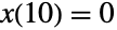

pfun = ParametricNDSolveValue[{x''[t] - x'[t] + x[t] == 0, x[0] == 1, x'[0] == s}, x[10], {t, 0, 10}, {s}];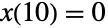
root = FindRoot[pfun[s] == 0, {s, 6}]NDSolve[{x''[t] - x'[t] + x[t] == 0, x[0] == 1, x'[0] == s} /. root, x, {t, 0, 10}];Plot[x[t] /. %, {t, 0, 10}]psol = ParametricNDSolveValue[{x''[t] - x'[t] + x[t] == 0, x[0] == 1, x'[0] == s}, x, {t, 0, 10}, {s}];Show[Plot[Evaluate@Table[Tooltip[psol[s][t], s], {s, 1, 1.8, 0.1}], {t, 0, 10}, PlotStyle -> Lighter[Gray, 0.5]],
Plot[psol[s][t] /. root, {t, 0, 10}, PlotStyle -> Orange]]境界値問題  ,
 ,
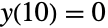 のいくつかの解を求める.まず,
 の可能な値をいくつか考える:
psol = ParametricNDSolveValue[{y''[t] + Sin[y[t]] == 0, y[0] == 0, y'[0] == s}, y, {t, 0, 10}, {s}];Plot[Evaluate@Table[Tooltip[psol[s][t], s], {s, 0.3, 1.9, 0.1}], {t, 0, 10}]
pfun = ParametricNDSolveValue[{y''[t] + Sin[y[t]] == 0, y[0] == 0, y'[0] == s}, y[10], {t, 0, 10}, {s}];Plot[pfun[s], {s, 0, 2.1}]val = Table[FindRoot[pfun[s], {s, s0}], {s0, {0.9, 1.9, 2}}]Plot[Evaluate[psol[s][t] /. val], {t, 0, 10}]古典的調和振動子  について,
 のすべての固有値とすべての固有関数
 を
 で求める.可能なパラメータ値を探ることから始める:
psol = ParametricNDSolveValue[{y''[x] == -λ^2 y[x], y[0] == 0, y'[0] == λ}, y, {x, 0, 1}, {λ}];Plot[Evaluate@Table[Tooltip[psol[λ][x], λ], {λ, π / 2, 11π / 2, π / 2}], {x, 0, 1}]
pfun = ParametricNDSolveValue[{y''[x] == -λ^2 y[x], y[0] == 0, y'[0] == λ}, y[1], {x, 0, 1}, {λ}];Plot[pfun[λ], {λ, π / 2, 11π / 2}]sol = Table[FindRoot[pfun[λ] == 0, {λ, λ0}], {λ0, {3, 6, 9, 12, 16}}]//QuietPlot[Evaluate[psol[λ][x] /. sol], {x, 0, 1}]量子的な調和振動子の最初の3つの固有関数, ,
 ,
 を求める.まず,
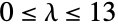 についての
 の解をプロットする:
pfun = ParametricNDSolveValue[{-y''[x] + x ^ 2 y[x] == λ y[x], y[0] == 0, y'[0] == 1}, y, {x, -15, 15}, {λ}];Plot[Evaluate@Table[pfun[λ][x], {λ, 0, 13, 1}], {x, -5, 5}, PlotRange -> {-2, 2}]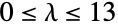

Plot[pfun[λ][5]Exp[-5], {λ, 0, 13}, PlotRange -> {-7, 7}]Map[FindRoot[pfun[λ][5], {λ, #}]&, {2.8, 6.5, 10}]
Show[Plot[Evaluate@Table[pfun[λ][x], {λ, 0, 13, 1}], {x, -5, 5}, PlotRange -> {-1, 1}, PlotStyle -> Lighter[Gray, .5]], Plot[{pfun[3][x], pfun[7][x], pfun[11][x]}, {x, -5, 5}]]両者は厳密な固有関数であるエルミート関数と倍率が異なるだけである:
ψ[n_, x_] := (HermiteH[n, x] E^-(x^2/2)/Sqrt[2^n n! Sqrt[π]])Plot[{ψ[1, x], -ψ[3, x], ψ[5, x]}, {x, -5, 5}, PlotRange -> {-1, 1}] ,
 の解が
 から
 までの最小弧長になるような
 の値を求める.0から1までの
 の値についての解をプロットすることから始める:
pfun = ParametricNDSolveValue[{y''[t] + y[t] == 3a Sin[y[t]], y[0] == y'[0] == 1, α'[t] == Sqrt[1 + y[t] ^ 2], α[0] == 0}, {y[t]}, {t, 0, 10}, {a}];
alfun = ParametricNDSolveValue[{y''[t] + y[t] == 3a Sin[y[t]], y[0] == y'[0] == 1, α'[t] == Sqrt[1 + y[t] ^ 2], α[0] == 0}, α[10], {t, 0, 10}, {a}];Plot[Evaluate@Table[Tooltip[pfun[a], a], {a, 0, 1, .1}], {t, 0, 10}]
Plot[alfun[a], {a, 0, 1}, MaxRecursion -> 0, PlotPoints -> 100]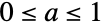

Show[Plot[Evaluate@Table[pfun[a], {a, 0, 1, .1}], {t, 0, 10}, PlotRange -> All, PlotPoints -> 500, PlotStyle -> Lighter[Gray, 0.3]], Plot[pfun[0], {t, 0, 10}, PlotStyle -> Thick]]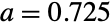
lmin = FindMinimum[alfun[a], {a, 0.725}, AccuracyGoal -> 7](局地的)最小弧長に対応する解をいくつかの近傍の解と一緒にプロットする:
Show[Plot[Evaluate@Table[pfun[a], {a, .65, .8, .005}], {t, 0, 10}, PlotRange -> All, PlotPoints -> 500, PlotStyle -> Lighter[Gray, 0.3]], Plot[pfun[a] /. lmin[[2]], {t, 0, 10}, PlotStyle -> Thick]]クライン・ゴルドン方程式の放射状形を の形のポテンシャルについて解く:
sol = ParametricNDSolveValue[{Derivative[2][R][r] - ((1 - (UnitConvert[Quantity[1, "FineStructureConstant"]] E^-r Z + ϵ)^2) R[r]) == 0, R[0] == 0, R'[0] == 1}, R, {r, 0, 50}, {ϵ, Z}]解  を外側の境界で減衰させるエネルギー
 と強度パラメータ
 の値をプロットする:
ContourPlot[sol[ϵ, Z][50] == 0, {Z, 50, 800}, {ϵ, -1, 1}, FrameLabel -> Automatic, PlotPoints -> 100]時間  における電圧v1でのステップに対するRLC回路の応答のシミュレーションを行う:
Subscript[v, 1][t_] := (Sign[t - .01] + 1) / 2;components = {r iR[t] == Subscript[v, 2][t] - Subscript[v, 3][t], l iL'[t] == Subscript[v, 1][t] - Subscript[v, 2][t], iC[t] == c Subscript[v, 3]'[t]};
connections = {iV[t] - iL[t] == 0, iL[t] - iR[t] == 0, iR[t] - iC[t] == 0};
ic = {iR[0] == 0, iL[0] == 0, iC[0] == 0, Subscript[v, 2][0] == 0, Subscript[v, 3][0] == 0};pfun = ParametricNDSolveValue[{components, connections, ic}, Subscript[v, 2], {t, 0, .03}, {r, l, c}];step = Plot[Subscript[v, 1][t], {t, 0, .03}, Filling -> {1 -> 0}, Ticks -> {Range[0.01, 0.03, 0.01], Automatic}]Show[step, Plot[Evaluate@Table[pfun[r, 10^-2, 10^-4][t], {r, {5, 10, 20, 40}}], {t, 0, .03}], PlotRange -> All]Show[step, Plot[Evaluate@Table[pfun[10, 10^-2l, 10^-4][t], {l, {.25, 1, 2}}], {t, 0, .03}], PlotRange -> All]Show[step, Plot[Evaluate@Table[pfun[10, 10^-2, 10^-4c][t], {c, {.25, 1, 2}}], {t, 0, .03}], PlotRange -> All]パラメータ感度 (5)
微分方程式のパラメータに摂動を与え,結果の摂動解をいくつか観察する:
pfun = ParametricNDSolveValue[{y''[t] + y[t] == a Sin[2t ] + Cos[2y[t]], y[0] == 1, y'[0] == 0}, y, {t, 0, 10}, {a}];Show[Plot[Evaluate@Table[pfun[a][t], {a, -.6, .6, .1}], {t, 0, 5}, PlotStyle -> Lighter[Gray, 0.3], PlotRange -> All], Plot[pfun[0][t], {t, 0, 5}]]Plot[Evaluate[pfun[0][t] + {-.5, 0, .5}pfun'[0][t]], {t, 0, 5}, PlotStyle -> {Gray, {Blue}, Gray}, Filling -> {1 -> {3}}]振動数 ω,振幅aで振動している台座上の安定した倒立振子のシミュレーションを行う:
pfun = ParametricNDSolveValue[{θ''[t] + (9.8 / 10)Sin[θ[t]] == -(a / 10)ω ^ 2 Sin[ω t]Sin[θ[t]], θ[0] == 3.14158, θ'[0] == 0.01}, θ, {t, 0, 5}, {ω, a}]; で
 のとき,振子は倒立位置
 近くで安定しているが,感度は上昇する:
if = pfun[50, 2];
ifa = D[pfun[ω, a], a] /. {ω -> 50, a -> 2};Plot[Evaluate[if[t] + {-.1, 0, .1}ifa[t]], {t, 0, 5}, PlotStyle -> {Gray, Blue, Gray}, Filling -> {1 -> {3}}]ndf = ParametricNDSolveValue[{Derivative[1][x][t] == -3 (x[t] - y[t]), Derivative[1][y][t] == -x[t] z[t] + a x[t] - y[t], Derivative[1][z][t] == x[t] y[t] - z[t], x[0] == z[0] == 0, y[0] == 1}, x[T], {t, 0, T}, {a, T}, MaxSteps -> ∞];Plot[Evaluate[RealExponent[D[ndf[a, 8], a]]], {a, 26, 27}, PlotRange -> All]

pfun = ParametricNDSolveValue[{D[u[t, x], t] == c^2 D[u[t, x], x, x], u[0, x] == Exp[-(a x) ^ 2], u[t, -10] == u[t, 10] == 0}, u, {t, 0, 5}, {x, -10, 10}, {a, c}];

ifun = pfun[1, 1];
ifda = D[pfun[a, 1], a] /. {a -> 1};
ifdc = D[pfun[1, c], c] /. {c -> 1};Panel@Grid[Join[{{"", "a", "c"}}, Table[{Row[{"t=", τ}], Plot[Evaluate[(ifun[τ, x] + .5{0, 1, -1}ifda[τ, x])], {x, -10, 10}, Filling -> {2 -> {3}}, PlotRange -> All], Plot[Evaluate[(ifun[τ, x] + .5{0, 1, -1}ifdc[τ, x])], {x, -10, 10}, Filling -> {2 -> {3}}, PlotRange -> All]}, {τ, {1, 3, 5}}]]]ColorSensitivityPlot3D[f_, fsense_, opts___] :=
Block[{fs = fsense}, Plot3D[f, {t, 0, 5}, {x, -10, 10}, Mesh -> None, ColorFunction -> Function[{t, x}, ColorData["LakeColors"][fs]], PlotPoints -> 60, ColorFunctionScaling -> False, opts]]{ColorSensitivityPlot3D[pfun[1, 1][t, x], 1.5Abs[ifda[t, x]], PlotLabel -> a, PlotRange -> All], ColorSensitivityPlot3D[pfun[1, 1][t, x], Abs[ifdc[t, x]], PlotLabel -> c, PlotRange -> All]}

pfun = ParametricNDSolveValue[{D[u[t, x], t, t] == c ^ 2 D[u[t, x], x, x], u[0, x] == Exp[-(a x) ^ 2], Derivative[1, 0][u][0, x] == 0, u[t, -10] == u[t, 10]}, u, {t, 0, 5}, {x, -10, 10}, {a, c}];

ifun = pfun[1, 1];
ifda = D[pfun[a, 1], a] /. {a -> 1};
ifdc = D[pfun[1, c], c] /. {c -> 1};Panel@Grid[Join[{{"", "a", "c"}}, Table[{StringJoin["t = ", ToString[τ]], Plot[Evaluate[(pfun[a, c][τ, x] + .5{0, 1, -1}D[pfun[a, c][τ, x], a]) /. {a -> 1, c -> 1}], {x, -10, 10}, Filling -> {2 -> {3}}, PlotRange -> All], Plot[Evaluate[(pfun[a, c][τ, x] + .5{0, 1, -1}D[pfun[a, c][τ, x], c]) /. {a -> 1, c -> 1}], {x, -10, 10}, Filling -> {2 -> {3}}, PlotRange -> All]}, {τ, {1, 3, 5}}]]]ColorSensitivityPlot3D[f_, fsense_, opts___] :=
Block[{fs = fsense}, Plot3D[f, {t, 0, 5}, {x, -10, 10}, Mesh -> None, ColorFunction -> Function[{t, x}, ColorData["LakeColors"][fs]], PlotPoints -> 60, ColorFunctionScaling -> False, opts]]{ColorSensitivityPlot3D[pfun[1, 1][t, x], Abs[ifda[t, x]], PlotLabel -> a, PlotRange -> All], ColorSensitivityPlot3D[pfun[1, 1][t, x], .25Abs[ifdc[t, x]], PlotLabel -> c, PlotRange -> All]}パラメータのフィッティング (2)
{sol, samples} = NDSolve[{y''[t] == -9.8, y[0] == 1, y'[0] == 40, WhenEvent[Mod[t, .5] == 0, Sow[{t, y[t]}]]}, y, {t, 0, 10}]//Reap;
noisysamples = Map[({#[[1]], #[[2]] + RandomReal[{-10, 10}]})&, First@samples];ListPlot[noisysamples]pfun = ParametricNDSolveValue[{y''[t] == -w y[t], y[0] == a, y'[0] == b}, y, {t, 0, 10}, {w, a, b}];fit = FindFit[noisysamples, pfun[w, a, b][t], {{w, .1}, {a, 1}, {b, 1}}, t]Plot[pfun[w, a, b][t] /. fit, {t, 0, 10}, Epilog -> {Point@noisysamples}]pfun = ParametricNDSolveValue[{y''[t] == -g, y[0] == p, y'[0] == v}, y, {t, 0, 10}, {g, p, v}];fit = FindFit[noisysamples, pfun[g, p, v][t], {{g, 5}, {p, .5}, {v, .5}}, t]Plot[pfun[g, p, v][t] /. fit, {t, 0, 10}, Epilog -> {Point@noisysamples}]微分方程式の解がデータに最もよくフィットするパラメータを求める:
time = Quantity[{0, 25, 34, 42, 54, 63, 80, 89, 103, 115, 131, 145, 158, 175, 195, 213, 225, 250, 274, 298, 315, 335, 353, 387, 411, 440, 475, 492, 520, 530, 550, 560, 570, 585, 600, 610, 620, 630, 640, 647, 660, 670, 680, 690, 700, 710, 720, 730, 740, 750, 760, 770, 778, 790, 800, 810, 820, 830, 840, 850, 860, 870, 880, 890, 900, 910, 920, 930, 940, 950, 960, 970, 980, 990, 1000, 1010, 1020, 1030, 1040, 1050, 1060, 1070, 1080, 1090, 1100, 1110, 1120, 1130, 1140, 1150, 1160, 1170, 1180, 1190, 1200, 1210, 1220, 1230, 1240, 1250, 1260, 1270, 1280, 1300, 1340, 1356, 1380, 1418, 1725, 1740, 1825, 1890, 1955, 2022, 2077, 2160, 2244, 2320, 2408, 2473, 2613}, "Seconds"];
temp = Quantity[{210, 204, 200, 198, 196, 194, 192, 190, 188, 186, 184, 182, 180, 178, 176, 174, 172, 170, 168, 166, 164, 162, 160, 158, 156, 154, 152, 150, 150, 148, 148, 147, 146, 145, 144, 144, 144, 143, 143, 142, 142, 141, 141, 140, 140, 139.5, 139, 139, 138, 138, 137, 137, 136, 136, 136, 135, 135, 134, 134, 133, 133, 133, 132.5, 132, 132, 131, 131, 131, 130, 130, 129.5, 129, 129, 128.5, 128, 128, 128, 127.5, 127, 127, 126, 126, 126, 125.5, 125, 125, 124.5, 124, 124, 123.5, 123, 123, 122.5, 122, 122, 122, 121.5, 121, 121, 121, 120.5, 120.5, 120, 120, 119, 118, 117, 116, 111, 110.5, 109, 108, 107, 106, 105, 104, 103, 102, 101, 100, 99}, "DegreesFahrenheit"];
データをカルビンに変換し,最初と最後の(アンビエント)温度を求める:
tempK = UnitConvert[temp, "Kelvins"];
Subscript[tempK, 0] = QuantityMagnitude[First[tempK]];
Subscript[tempK, ∞] = QuantityMagnitude[UnitConvert[Quantity[79, "DegreesFahrenheit"], "Kelvins"]];
tend = QuantityMagnitude[Last[time]];パラメータk1とk2に依存する,ニュートンの冷却法則の解を求める:
BoltzmannConstant = Quantity[1.3806504`*^-23 , "Joules" / "Kelvins"];
c = QuantityMagnitude[(2260 18/6.02 10^23 BoltzmannConstant)];pfun = ParametricNDSolveValue[{(Derivative[1][T][t] == -k1(T[t] - Subscript[tempK, ∞]) - k2 (E^-c / T[t] - E^-c / Subscript[tempK, ∞])), T[0] == Subscript[tempK, 0]}, T, {t, 0, tend}, {k1, k2}];fitdata = N@QuantityMagnitude[Transpose[{time, tempK}]];fit = FindFit[fitdata, pfun[k1, k2][t], {{k1, 0.0001}, {k2, 10000}}, t]Show[ ListPlot[fitdata], Plot[Evaluate[pfun[k1, k2][t] /. fit], {t, 0, tend}, PlotStyle -> Red]]特性と関係 (3)
NDSolveValueを使ってパラメータを持つ微分方程式を解く:
ndsvfun[a_] := NDSolveValue[{y''[t] == -a y[t] + t Sin[y[t]], y[0] == 1, y'[0] == 1}, y, {t, 0, 100}];指定されたパラメータ値について,各関数の呼出しにはほぼ同じ時間がかかる:
Table[First@AbsoluteTiming[ndsvfun[1][100]], {10}]ParametricNDSolveは解をキャッシュし,キャッシュした解の値を再度使う:
pfun = ParametricNDSolveValue[{y''[t] == -a y[t] + t Sin[y[t]], y[0] == 1, y'[0] == 1}, y, {t, 0, 100}, {a}];Table[First@AbsoluteTiming[pfun[1][100]], {10}]DSolveは閉じた形のパラメータを持つ微分方程式を解くことができることもある:
dsol = y[x] /. First@DSolve[{y'[x] + a y[x] == 1, y[0] == 1}, y[x], x]ParametricNDSolveValueを使って例題を数値的に解く:
ndsol = ParametricNDSolveValue[{y'[x] + a y[x] == 1, y[0] == 1}, y, {x, 0, 5}, {a}, MaxStepSize -> 0.01];Plot[Evaluate[{D[dsol, a], D[ndsol[a][x], a]} /. a -> 1], {x, 0, 5}]SystemModelParametricSimulateを使って大きい階層的系のモデルのシミュレーションを行う:
pf = SystemModelParametricSimulate[\!\(\*GraphicsBox[«8»]\), "Inertia2.w", 40, {"Resistor1.R", "SpringDamper1.d"}]抵抗器とバネ減衰器のパラメータ2セットでシミュセーションを行う:
sims = {pf[0.1, 0.25], pf[0.4, 0.3]};Plot[Evaluate@Through[sims[t]], {t, 0, 40}]考えられる問題 (1)
WhenEvent,ReapおよびSowによる解のサンプリングは,各パラメータ値への最初の呼出しにのみ使うことができる:
pfun = ParametricNDSolveValue[{y''[t] == -a Cos[ y[t]], WhenEvent[Mod[t, 1], Sow[{t, y[t]}]], y[0] == 1, y'[0] == 1}, y, {t, 0, 10}, {a}]{ifun, {points}} = pfun[10]//ReapPlot[ifun[t], {t, 0, 10}, Epilog -> {PointSize[Medium], Red, Point[points]}]{ifun, points} = pfun[10]//ReapPlot[ifun[t], {t, 0, 10}, Epilog -> {PointSize[Medium], Red, Point[points]}]テキスト
Wolfram Research (2012), ParametricNDSolveValue, Wolfram言語関数, https://reference.wolfram.com/language/ref/ParametricNDSolveValue.html (2014年に更新).
CMS
Wolfram Language. 2012. "ParametricNDSolveValue." Wolfram Language & System Documentation Center. Wolfram Research. Last Modified 2014. https://reference.wolfram.com/language/ref/ParametricNDSolveValue.html.
APA
Wolfram Language. (2012). ParametricNDSolveValue. Wolfram Language & System Documentation Center. Retrieved from https://reference.wolfram.com/language/ref/ParametricNDSolveValue.html