QuadraticOptimization[{q,c},{a,b}]
線形不等式制約 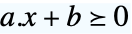 に従って二次目的関数
 を最小化するベクトル
 を求める.
QuadraticOptimization[{q,c},{a,b},{aeq,beq}]
線形等式制約 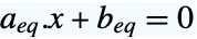 を含む.
QuadraticOptimization[{q,c},…,{dom1,dom2,…}]





QuadraticOptimization
QuadraticOptimization[f,cons,vars]
線形制約条件 cons に従って二次目的関数 f を最小化する変数 vars の値を求める.
QuadraticOptimization[{q,c},{a,b}]
線形不等式制約 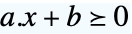 に従って二次目的関数
 を最小化するベクトル
 を求める.
QuadraticOptimization[{q,c},{a,b},{aeq,beq}]
線形等式制約 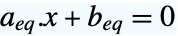 を含む.
QuadraticOptimization[{q,c},…,{dom1,dom2,…}]

QuadraticOptimization[…,"prop"]
解のどの特性"prop"を返すべきかを指定する.
詳細とオプション
- 二次最適化は,二次計画法(QP),混合整数二次計画法(MIQP),あるいは線形制約二次最適化としても知られている.
- 二次最適化は,パラメータのフィット,ポートフォリオの最適化,幾何学的距離問題等によく使われる.
- 二次最適化は,実変数,整数変数あるいは複素変数で大域的に効率よく解くことができる凸最適化問題である.
- 二次最適化は主問題を解く
 を求める. »
-
最小化 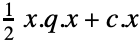
制約条件 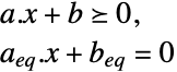
ただし 
- 空間
 は対称正定値行列からなる.
- 混合整数の二次最適化は,問題を解く
 および
 を求める.
-
最小化 
制約条件 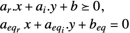
ただし 
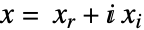
- QuadraticOptimizationは,目的関数が実数値のときは,内部的に実変数
 に変換して
 の問題を解く.ただし,
 で
 である.
- 変数指定 vars は,次のいずれかの形式で変数を与える要素のリストでなければならない.
-
v 名前が  で次元が推測される変数
v∈Reals 実数のスカラー変数 v∈Integers 整数のスカラー変数 v∈Complexes 複素数のスカラー変数 v∈ℛ 幾何学領域  に制限されたベクトル変数
v∈Vectors[n,dom]  または
 のベクトル変数
v∈Matrices[{m,n},dom]  または
 の行列変数
- 制約条件 cons は以下で指定できる.
-
LessEqual 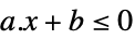
スカラー不等式 GreaterEqual 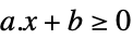
スカラー不等式 VectorLessEqual 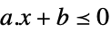
ベクトル不等式 VectorGreaterEqual 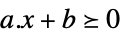
ベクトル不等式 Equal 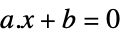
スカラー等式またはベクトル等式 Element 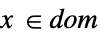
凸領域または領域要素 - QuadraticOptimization[f,cons,vars]のとき,f または cons に使われるパラメータを定義するために,parval の形式のパラメータ方程式が制約条件に含まれることがある.ただし,par は vars に含まれず,val は数値または数値配列である.
- 目的関数は次の方法で指定できる.
-
q 
{q,c} 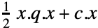


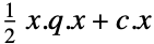
- 因数分解した形式では,
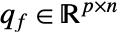 と
 である.
- 主最小化問題には関連したラグランジュ双対問題である最大化問題がある.双対最大値は常に主最小値以下である.したがって,これは下界を与える.双対マキシマイザは主問題についての,最小値の感度や制約条件の変更等を含む情報を与える.
- 目的関数が
 の二次最適化についてのラグランジュ双対問題は以下で与えられる. »
-
最大化 
制約条件 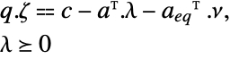
ただし 
- 因数分解された二次目的関数が
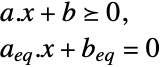 のとき,双対問題は次のように表すことができる.
-
最大化 
制約条件 
ただし 
- 因数分解された双対ベクトル
 と因数分解されていない双対ベクトル
 の関係は
 である.
- 二次最適化では,
 が半正定値の場合は強双対性が成り立つ.したがって,主最小化問題に解があれば双対最大化問題にも解があり,双対最大値と主最小値は等しい.
- 使用可能な解の特性"prop"には以下がある.
-
"PrimalMinimizer" 
目的関数を最小化する変数値のリスト "PrimalMinimizerRules" 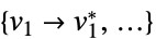
 を最小化する変数の値 vars={v1,…}
"PrimalMinimizerVector" 
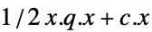 を最小化するベクトル
"PrimalMinimumValue" 
最小値 
"DualMaximizer" 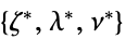
 を最大化するベクトル
"DualMaximumValue" 
双対最大値 "DualityGap" 
双対最適値と主最適値の差(強双対性のため0) "Slack" 
制約条件の摂動に対する感度 "ConstraintSensitivity" 
最小値の制約条件に対する感度 
"ObjectiveMatrix" 
二次目的行列 "ObjectiveVector" 
線形目的ベクトル "FactoredObjectiveMatrix" 
因数分解された目的形式の行列 "FactoredObjectiveVector" 
因数分解された目的形式のベクトル "LinearInequalityConstraints" 
線形不等式制約行列と線形不等式制約ベクトル "LinearEqualityConstraints" 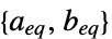
線形等式制約行列と線形等式制約ベクトル {"prop1","prop2",…} いくつかの解の特性 - 双対マキシマイザの成分
 は,
 で与えられる
 と
 の関数である.
- 次は,使用可能なオプションである.
-
MaxIterations Automatic 使用する最大反復回数 Method Automatic 使用するメソッド PerformanceGoal $PerformanceGoal パフォーマンスのどの局面について最適化するか Tolerance Automatic 内部比較の許容度 WorkingPrecision MachinePrecision 内部計算精度 - オプション Method->method を使って使用するメソッドを指定することができる.次は,使用可能なメソッドである.
-
Automatic 自動的にメソッドを選択する "COIN" COIN ライブラリ二次計画法 "SCS" SCS(分割円錐ソルバ)ライブラリ "OSQP" 二次問題のためにソルバを分割するOSQP演算子 "CSDP" CSDP(COIN半定値計画法)ライブラリ "DSDP" DSDP(半定値計画法)ライブラリ "PolyhedralApproximation" 客観的なエピグラフは多面体を使って近似される "MOSEK" 商用MOSEK凸最適化ソルバ "Gurobi" 商用Gurobi線形・二次最適化ソルバ "Xpress" 商用Xpress線形・二次最適化ソルバ
例題
すべて開く すべて閉じる例 (3)
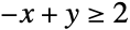

obj = 2x^2 + 20y^2 + 6x y + 5x;
res = QuadraticOptimization[obj, -x + y ≥ 2, {x, y}]
Show[Plot3D[obj, {x, -2, 0}, {y, 0, 1}, ...], Graphics3D[{Blue, PointSize[0.05], Point[{x, y, obj} /. res]}]]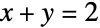
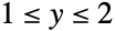

res = QuadraticOptimization[x^2 + y^2, {x + y == 2, 1 ≤ y ≤ 2}, {x, y}]

{q, c} = {{{2, 0}, {0, 2}}, {0, 0}};
{a, b} = {{{0, 1}, {0, -1}}, {-1, 2}};
{aeq, beq} = {{{1, 1}}, {-2}};QuadraticOptimization[{q, c}, {a, b}, {aeq, beq}]
Show[RegionPlot[Evaluate[x^2 + y^2 ≤ (x^2 + y^2 /. res)], ...], ContourPlot[x + y == 2, {x, 0.5, 1.5}, {y, 0.5, 1.5}, ContourStyle -> Red]]

obj = 2x^2 + 20y^2 + 6x y + 5x;
res = QuadraticOptimization[obj, -x + y ≥ 2, {x∈Integers, y∈Reals}]{q, c} = {{{4, 6}, {6, 40}}, {5, 0}};
{a, b} = {{{-1, 1}}, {-2}};
QuadraticOptimization[{q, c}, {a, b}, {Integers, Reals}]スコープ (26)
基本的な用法 (8)
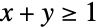

QuadraticOptimization[x^2 + y^2, x + y ≥ 1, {x, y}]解の特性"PrimalMinimumValue"を使って最小にする値を得る:
QuadraticOptimization[x^2 + y^2, x + y ≥ 1, {x, y}, "PrimalMinimumValue"]

QuadraticOptimization[2x^2 + 20y^2 + 6x y + 5x, {-x + y ≥ 2, y ≥ 0}, {x, y}]QuadraticOptimization[2x^2 + 20y^2 + 6x y + 5x, {-x + y ≥ 2, y ≥ 0}, {x, y}, {"PrimalMinimumValue", "PrimalMinimizer"}]

QuadraticOptimization[x^2 + y^2, {x + y ≤ 2, 1 ≤ y ≤ 2}, {x, y}]
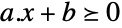
{q, c} = {{{2, 0}, {0, 2}}, {0, 0}};
{a, b} = {{{-1, -1}, {0, 1}, {0, -1}}, {2, -1, 2}};QuadraticOptimization[{q, c}, {a, b}]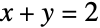
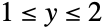

QuadraticOptimization[x^2 + y^2, {x + y == 2, 1 ≤ y ≤ 2}, {x, y}]
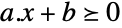

{q, c} = {{{2, 0}, {0, 2}}, {0, 0}};
{a, b} = {{{0, 1}, {0, -1}}, {-1, 2}};
{Subscript[a, eq], Subscript[b, eq]} = {{{1, 1}}, {-2}};QuadraticOptimization[{q, c}, {a, b}, {Subscript[a, eq], Subscript[b, eq]}]

QuadraticOptimization[2x^2 + 5y^2 + 4x y, {x + y ≥ 1, x - 2y ≤ 0}, {x, y}]
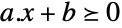
{qf, c} = {Sqrt[2] * {{1, 0}, {0, 1}, {1, 2}}, {0, 0}};
{a, b} = {{{1, 1}, {-1, 2}}, {-1, 0}};QuadraticOptimization[{{qf}, c}, {a, b}]

QuadraticOptimization[2x^2 + 5y^2 + 4x y, {x + y ≥ 1, x - 2y ≤ 0, 0 ≤ x ≤ 1, -1 ≤ y ≤ 1}, {x, y}]VectorGreaterEqual ()とVectorLessEqual ()を使って制約条件 を指定する:
QuadraticOptimization[2x^2 + 5y^2 + 4x y, {x + y ≥ 1, x - 2y ≤ 0, {0, -1}{x, y}{1, 1}}, {x, y}]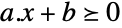 に従って
 を最小化する.ベクトル変数と定数パラメータ方程式を使う:
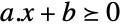
peqns = {q == {{2, 2}, {2, 5}}, a == {{1, 1}, {-1, 2}, {1, 0}, {0, 1}}, b == {-1, 0, 0, 0}};QuadraticOptimization[x.q.x, {peqns, a.x + b0}, x] に従って
 を最小化する.NonNegativeRealsを使って制約条件
 を指定する:
peqns = {q == {{2, 2}, {2, 5}}, a == {{1, 1}, {-1, 2}}, b == {-1, 0}};QuadraticOptimization[x.q.x, {peqns, a.x + b0}, x∈Vectors[2, NonNegativeReals]]整数変数 (4)
Integersを使って整数領域制約を指定する:
QuadraticOptimization[2x^2 + 5y^2 + 4x y, {x + y ≥ 1, x - 2y ≤ 0, 0 ≤ x ≤ 1, -1 ≤ y ≤ 1}, {x∈Integers, y∈Integers}]Vectors[n,Integers]を使ってベクトル変数についての整数領域制約を指定する:
peqns = {q == {{2, 2}, {2, 5}}, a == {{1, 1}, {-1, 2}}, b == {-1, 0}};QuadraticOptimization[x.q.x, {peqns, a.x + b0}, x∈Vectors[2, Integers]]NonNegativeIntegers ( )を使って非負の整数領域制約を指定する:
peqns = {q == {{2, 2}, {2, 5}}, a == {{1, 1}, {-1, 2}}, b == {-1, 0}};QuadraticOptimization[x.q.x, {peqns, a.x + b0}, x∈Vectors[2, NonNegativeIntegers]]NonPositiveIntegers ( )を使って非正の整数制約を指定する:
peqns = {q == {{2, 4}, {4, 8}}, a == {{1, 1}, {-1, 2}}, b == {5, 0}};QuadraticOptimization[x.q.x, {peqns, a.x + b0}, x∈Vectors[2, NonPositiveIntegers]]複素変数 (3)
Complexesを使って複素変数を指定する:
QuadraticOptimization[Inactive[Norm][{x, y}] ^ 2, {xI, y1}, {x∈Complexes, y∈Complexes}]

{q, c} = {{{2, 1 + I}, {1 - I, 1}}, {2, 3}};
QuadraticOptimization[(1 / 2) * x.q.x + c.x, {}, x∈Vectors[2, Reals]]

q = {{1, I}, {-I, 2}};
QuadraticOptimization[(1 / 2) * Inactive[Dot][Conjugate[x], q, x] , {{1, I}.x1 + I}, x∈Vectors[2, Complexes]]主モデルの特性 (4)
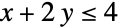

QuadraticOptimization[(x - 1)^2 + (y - 5 / 2)^2 - (3 / 2)^2, x + 2y ≤ 4, {x, y}]"PrimalMinimizer"を使ってベクトル出力を得る:
QuadraticOptimization[(x - 1)^2 + (y - 5 / 2)^2 - (3 / 2)^2, x + 2y ≤ 4, {x, y}, "PrimalMinimizer"]"PrimalMinimizerRules"を使ってルールベースの結果を得る:
QuadraticOptimization[(x - 1)^2 + (y - 5 / 2)^2 - (3 / 2)^2, x + 2y ≤ 4, {x, y}, "PrimalMinimizerRules"]"PrimalMinimumValue"を使って最適化の最小にする値を得る:
QuadraticOptimization[(x - 1)^2 + (y - 5 / 2)^2 - (3 / 2)^2, x + 2y ≤ 4, {x, y}, "PrimalMinimumValue"]obj = (x - 1)^2 + (y - 5 / 2)^2 - (3 / 2)^2;
cons = x + 2y ≤ 4;Subscript[p, sym] = QuadraticOptimization[obj, cons, {x, y}, "PrimalMinimumValue"]{q, c, {a, b}} = QuadraticOptimization[obj, cons, {x, y}, {"ObjectiveMatrix", "ObjectiveVector", "LinearInequalityConstraints"}];Subscript[p, m] = QuadraticOptimization[{q, c}, {a, b}, "PrimalMinimumValue"]const = QuadraticOptimization[obj, cons, {x, y}, "ObjectiveConstant"]Subscript[p, sym] == Subscript[p, m] + constobj = 2x^2 + 20y^2 + 6x y + 5x;
cons = {-x + y ≥ 2, x + y == 1, y ≥ 1};{Subscript[s, ineq], Subscript[s, eq]} = QuadraticOptimization[obj, cons, {x, y}, "Slack"]{x^ * , {a, b}, {Subscript[a, eq], Subscript[b, eq]}} = QuadraticOptimization[obj, cons, {x, y}, {...}];不等式制約 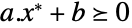 についてのスラックは,
 となるようなベクトル
 である:
Norm[a.x^ * + b - Subscript[s, ineq]] == 0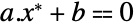


Norm[Subscript[a, eq].x^ * + Subscript[b, eq] - Subscript[s, eq]] == 0
Subscript[s, eq]//Chop双対モデルの特性 (3)
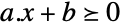


{q, c} = {{{2, 0}, {0, 2}}, {1, 1}};
{a, b} = {{{-1, 1}, {0, 1}}, {-2, -1}};
{Subscript[a, eq], Subscript[b, eq]} = {{{1, 1}}, {-1}};
xv = Table[Indexed[x, i], {i, 2}];psol = QuadraticOptimization[(xv.q.xv) / 2 + c.xv, {a.xv + b0, Subscript[a, eq].xv + Subscript[b, eq] == 0}, xv]

{ζv, λv, νv} = {Table[Indexed[ζ, i], {i, 2}], Table[Indexed[λ, i], {i, 2}], Table[Indexed[ν, i], {i, 1}]};dsol = QuadraticOptimization[(ζv.q.ζv) / 2 + b.λv + Subscript[b, eq].νv, {q.ζv + a.λv + Subscript[a, eq].νv == c, λv0}, Join[ζv, λv, νv]]{(xv.q.xv) / 2 + c.xv /. psol, -((ζv.q.ζv) / 2 + b.λv + Subscript[b, eq].νv) /. dsol}したがって,双対性ギャップはゼロである.一般に,最適点で である:
QuadraticOptimization[(xv.q.xv) / 2 + c.xv, {a.xv + b0, Subscript[a, eq].xv + Subscript[b, eq] == 0}, xv, "DualityGap"]obj = x ^ 2 + y ^ 2 + x + y;
constraints = {-x + y ≥ 2, y ≥ 1, x + y == 1};QuadraticOptimization[obj, constraints, {x, y}]{q, c, {a, b}, {Subscript[a, eq], Subscript[b, eq]}} = QuadraticOptimization[obj, constraints, {x, y},
{"ObjectiveMatrix", "ObjectiveVector", "LinearInequalityConstraints", "LinearEqualityConstraints"}];

QuadraticOptimization[((ζ.q.ζ) / 2 + b.λ + Subscript[b, eq].ν), {q.ζ + a.λ + Subscript[a, eq].ν == c, λ0}, {ζ, λ, ν}]QuadraticOptimization[x ^ 2 + y ^ 2 + x + y, {-x + y ≥ 2, y ≥ 1, x + y == 1}, {x, y}, "DualMaximumValue"]QuadraticOptimization[x ^ 2 + y ^ 2 + x + y, {-x + y ≥ 2, y ≥ 1, x + y == 1}, {x, y}, "DualMaximizer"]感度特性 (4)
"ConstraintSensitivity"を使って,制約緩和による最適値の変化を求める:
{q, c} = {{{2, 0}, {0, 2}}, {0, 0}};
{a, b} = {{{-1, -1}, {-1, 2}}, {-1, 0}};
p^ * = QuadraticOptimization[{q, c}, {a, b}, "PrimalMinimumValue"];{Subscript[s, λ], Subscript[s, ν]} = QuadraticOptimization[{q, c}, {a, b}, "ConstraintSensitivity"]

δb = {0.01, 0.01};p^ * + δb.Subscript[s, λ]QuadraticOptimization[{q, c}, {a, b + δb}, "PrimalMinimumValue"]{Subscript[s, λ], Subscript[s, ν]} = QuadraticOptimization[x^2 + y^2 + z^2 - 2x - 6y + z, {x + 2y ≥ 4, x ≤ 3, x + y + z == 1, x - y == 2}, {x, y, z}, "ConstraintSensitivity"]{{a, b}, {Subscript[a, eq], Subscript[b, eq]}} = QuadraticOptimization[x^2 + y^2 + z^2 - 2x - 6y + z, {x + 2y ≥ 4, x ≤ 3, x + y + z == 1, x - y == 2}, {x, y, z}, {"LinearInequalityConstraints", "LinearEqualityConstraints"}];Table[{a[[i]].{x, y, z} + b[[i]] ≥ 0, Subscript[s, λ][[i]]}, {i, 2}]Table[{Subscript[a, eq][[i]].{x, y, z} + Subscript[b, eq][[i]] == 0, Subscript[s, ν][[i]]}, {i, 2}]q = {{2, 0, 0}, {0, 2, 0}, {0, 0, 2}};
c = {-2, -6, 1};
{a, b} = {{{1, 2, 0}, {-1, 0, 0}}, {-4, 3}};
{Subscript[a, eq], Subscript[b, eq]} = {{{1, 1, 1}, {1, -1, 0}}, {-1, -2}};{p^ * , {Subscript[s, λ], Subscript[s, ν]}} = QuadraticOptimization[{q, c}, {a, b}, {Subscript[a, eq], Subscript[b, eq]}, {"PrimalMinimumValue", "ConstraintSensitivity"}]Subscript[s, λ][[2]]Chop[p^ * - QuadraticOptimization[{q, c}, {a, b + {0, 0.01}}, {Subscript[a, eq], Subscript[b, eq]}, "PrimalMinimumValue"]] == 0Subscript[s, λ][[1]]p^ * > QuadraticOptimization[{q, c}, {a, b + {0.1, 0}}, {Subscript[a, eq], Subscript[b, eq]}, "PrimalMinimumValue"]Subscript[s, ν][[1]]p^ * < QuadraticOptimization[{q, c}, {a, b}, {Subscript[a, eq], Subscript[b, eq] + {0.1, 0}}, "PrimalMinimumValue"]"ConstraintSensitivity"は,問題の双対マキシマイザに関連している:
{{Subscript[s, λ], Subscript[s, ν]}, {ζ, λ^ * , ν^ * }} = QuadraticOptimization[x^2 + y^2 + z^2 - 2x - 6y + z, {x + 2y ≥ 4, x ≤ 3, x + y + z == 1, x - y == 2}, {x, y, z}, {"ConstraintSensitivity", "DualMaximizer"}]不等式感度  は
 を満足する.ただし,
 は双対不等式マキシマイザである:
Subscript[s, λ] == -λ^ *等式感度 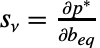 は
 を満足する.ただし,
 は双対等式マキシマイザである:
Subscript[s, ν] == -ν^ *オプション (12)
Method (5)
obj = 2x^2 + 20y^2 + 6x y + 5x;
cons = {-x + y ≥ 2, y ≥ 1};QuadraticOptimization[obj, cons, {x, y}, Method -> "COIN"]QuadraticOptimization[obj, cons, {x, y}, Method -> "CSDP"]QuadraticOptimization[obj, cons, {x, y}, Method -> "DSDP"]QuadraticOptimization[obj, cons, {x, y}, Method -> "SCS"]"PolyhedralApproximation"は線形制約を使ってオブジェクトを近似する:
QuadraticOptimization[obj, cons, {x, y}, Method -> "PolyhedralApproximation"]最小二乗型の二次問題については,"CSDP"と"DSDP"は"COIN"または"SCS"よりも低速である:
SeedRandom[123];
mat = RandomReal[{-1, 1}, {400, 10}];
rhs = RandomReal[{-1, 1}, 400];AbsoluteTiming[Subscript[x, COIN] = QuadraticOptimization[{{mat, -rhs}, {}}, {}, Method -> "COIN"];]AbsoluteTiming[Subscript[x, CSDP] = QuadraticOptimization[{{mat, -rhs}, {}}, {}, Method -> "CSDP"];]Norm[Subscript[x, COIN] - Subscript[x, CSDP]]最小二乗型の二次問題については,"CSDP","DSDP","PolyhedralApproximation"は"COIN"あるいは"SCS"よりも遅い:
SeedRandom[123];
mat = RandomReal[{-1, 1}, {40, 10}];
rhs = RandomReal[{-1, 1}, 40];
Subscript[x, Ref] = LeastSquares[mat, rhs];AbsoluteTiming[Subscript[x, COIN] = QuadraticOptimization[{{mat, -rhs}, {}}, {}, Method -> "COIN"];]Norm[Subscript[x, COIN] - Subscript[x, Ref]]AbsoluteTiming[Subscript[x, CSDP] = QuadraticOptimization[{{mat, -rhs}, {}}, {}, Method -> "CSDP"];]Norm[Subscript[x, CSDP] - Subscript[x, Ref]]"PolyhedralApproximation"法を使って問題を解く:
AbsoluteTiming[Subscript[x, PA] = QuadraticOptimization[{{mat, -rhs}, {}}, {}, Method -> "PolyhedralApproximation"];]Norm[Subscript[x, PA] - Subscript[x, Ref]]複数の最適解がある問題については,メソッドによって結果が異なることがある:
QuadraticOptimization[x ^ 2, {0 ≤ x ≤ 1}, {x, y}, Method -> "SCS"]QuadraticOptimization[x ^ 2, {0 ≤ x ≤ 1}, {x, y}, Method -> "COIN"]QuadraticOptimization[x ^ 2, {0 ≤ x ≤ 1}, {x, y}, Method -> "DSDP"]凹関数の最小化はMethod"COIN"を使ってのみ行うことができる:
QuadraticOptimization[-(x ^ 2), 0 ≤ x ≤ 1, x, Method -> "COIN"]QuadraticOptimization[-(x ^ 2), 0 ≤ x ≤ 1, x, Method -> "CSDP"]
PerformanceGoal (1)
"Quality"設定で計算時間を犠牲にし,より正確な結果を得る:
SeedRandom[123];
mat = RandomReal[{-1, 1}, {400, 10}];
rhs  = mat.RandomReal[{-1, 1}, 10];
{a, b} = {{UnitVector[10, 1]}, {0.1}};AbsoluteTiming[pQuality = QuadraticOptimization[{{mat, -rhs}, {}}, {a, b}, "PrimalMinimumValue", PerformanceGoal -> "Quality"];]AbsoluteTiming[pSpeed = QuadraticOptimization[{{mat, -rhs}, {}}, {a, b}, "PrimalMinimumValue", PerformanceGoal -> "Speed"];]{pQuality, pSpeed}Tolerance (2)
Toleranceの設定値を小さくすると,より正確な結果が得られる:
SeedRandom[123];
mat = RandomReal[{-1, 1}, {800, 10}];
rhs  = mat.RandomReal[{-1, 1}, 10];
Subscript[p, exact] = 0;Toleranceの設定値を変えて,計算上の最小値と厳密な最小値の誤差を求める:
err = Table[{tol, Abs[QuadraticOptimization[{{mat, -rhs}, {}}, {},
"PrimalMinimumValue", Tolerance -> tol, Method -> "SCS"] - Subscript[p, exact]]}, {tol, 10. ^ -Range[7]}]ListLogLogPlot[err, PlotRange -> All, Joined -> True, PlotMarkers -> Automatic]Toleranceの設定を小さくするとより正確な答が得られるが,計算時間は長くなることが多い:
SeedRandom[123];
mat = RandomReal[{-1, 1}, {500, 10}];
rhs = mat.RandomReal[{-1, 1}, 10];AbsoluteTiming[ptight = QuadraticOptimization[{{mat, -rhs}, {}}, {}, "PrimalMinimumValue", Method -> "CSDP", Tolerance -> 10 ^ -6];]AbsoluteTiming[ploose = QuadraticOptimization[{{mat, -rhs}, {}}, {}, "PrimalMinimumValue", Method -> "CSDP", Tolerance -> 10 ^ -3];]{ptight, ploose}WorkingPrecision (4)
MachinePrecisionは,QuadraticOptimizationにおけるWorkingPrecisionオプションのデフォルトである:
QuadraticOptimization[x^2 + y^2 - 2x - 3y, {x + 2 y ≤ 3}, {x, y}]QuadraticOptimization[x^2 + y^2 - 2x - 3y, {x + 2 y ≤ 3}, {x, y}, WorkingPrecision -> MachinePrecision]WorkingPrecisionAutomaticのとき,QuadraticOptimizationは使用する精度を入力から推測する:
QuadraticOptimization[x^2 + y^2 - 2x - 3y, {x + 2 y ≤ 3}, {x, y}, WorkingPrecision -> Automatic]QuadraticOptimizationは任意性度数を使って結果が計算できる:
QuadraticOptimization[x^2 + y^2 - 2x - 3y, {x + 2 y ≤ 3}, {x, y}, WorkingPrecision -> 20]指定された精度が入力引数の精度よりも低い場合は,メッセージが出される:
QuadraticOptimization[x^2 + y^2 - 2x - 3y, {x + 2 y ≤ N[3, 20]}, {x, y}, WorkingPrecision -> 30]

高精度の結果が計算できないときは,メッセージが出されてMachinePrecisionの結果が返される:
QuadraticOptimization[(1 + x + 2 y) (1 + x + y), {x + y ≤ -2, x + y ≤ 0}, {x, y}, WorkingPrecision -> Infinity]

アプリケーション (29)
基本的なモデリング変換 (7)
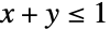 に従って
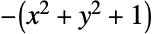 を最大化する.目的関数を否定することで最大化問題を解く:
QuadraticOptimization[(x^2 + y^2 + 1), x + y ≤ 1, {x, y}]-QuadraticOptimization[(x^2 + y^2 + 1), x + y ≤ 1, {x, y}, "PrimalMinimumValue"]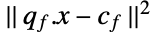

{qf, cf} = IconizedObject[«Block»];
q = Transpose[qf].qf;
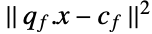
c = -2cf.qf;QuadraticOptimizationは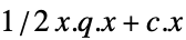 を最小化するので,行列は2倍される:
{Subscript[x, min], Subscript[g, min]} = QuadraticOptimization[{2q, c}, {}, {"PrimalMinimizer", "PrimalMinimumValue"}]
{Norm[qf.Subscript[x, min] - cf], Sqrt[Subscript[g, min] + cf.cf]}QuadraticOptimizationはこの変換を直接実行する.Inactiveを使って目的関数を構築することで縫込みを回避する:
QuadraticOptimization[Norm[Inactive[Plus][qf.x, -cf]], {}, x, {"PrimalMinimizer", "PrimalMinimumValue"}]制約条件  に従って
 を最小化する.目的関数を
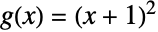 に変換して問題を解く:
QuadraticOptimization[(x + 1) ^ 2, {x + y ≤ 3, x ≥ 1, y ≥ 1}, {x, y}]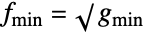
minval = QuadraticOptimization[(x + 1) ^ 2, {x + y ≤ 3, x ≥ 1, y ≥ 1}, {x, y}, "PrimalMinimumValue"]Sqrt[minval]制約条件 に従って
 を最小化する.制約条件は
 に変換することができる:
QuadraticOptimization[(x + y) ^ 2, {-3 ≤ 2x + y ≤ 3, x ≥ 1, y ≥ 1}, {x, y}]制約条件 に従って
 を最小化する.制約条件
 は
 と解釈することができる.各制約条件でこの問題を解く:
res1 = QuadraticOptimization[(x + y) ^ 2, {2x + y ≥ 1, x ≤ 1, y ≥ 1}, {x, y}, {"PrimalMinimumValue", "PrimalMinimizer"}]res2 = QuadraticOptimization[(x + y) ^ 2, {2x + y ≤ -1, x ≤ 1, y ≥ 1}, {x, y}, {"PrimalMinimumValue", "PrimalMinimizer"}]First@MinimalBy[{res1, res2}, First] に従って
 を最小化する.ただし,
 は代りに
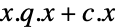 を最小化する非減少関数である.主ミニマイザは
 はどちらの問題でも同じままである.
 に従って
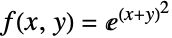 を最小化することを考える:
f = Function[{s}, Exp[s]];{minval, Subscript[X, min]} = QuadraticOptimization[(x + y) ^ 2, {2x - y ≥ 1, x ≥ 0, y ≥ 0}, {x, y}, {"PrimalMinimumValue", "PrimalMinimizerRules"}]
f[minval]

f = Function[{s}, Sqrt[s]];{minval, Subscript[X, min]} = QuadraticOptimization[3 + x + (x - y)^2, {2x + y ≥ 1, -2 ≤ y ≤ 2}, {x, y}, {"PrimalMinimumValue", "PrimalMinimizerRules"}] なので,主最小値が0より大きいときにのみ解は真の解である.主最小値は関数
 を主最小値に適用することで得られる:
f[minval]データフィッティング問題 (7)
data = IconizedObject[«Block»];
dataplot = ListPlot[data, PlotRange -> All]DesignMatrixを使って因数分解した二次行列を構築する:
qf = DesignMatrix[data, {1, x}, x];
cf = -data[[All, 2]];res = QuadraticOptimization[{{qf, cf}, 0}, {}]Show[dataplot, Plot[Evaluate[res.{1, x}], {x, 0, 1}]]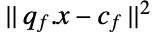
data = IconizedObject[«Block»];
dataplot = ListPlot[data, PlotRange -> All]DesignMatrixを使って因数分解した二次行列を構築する:
qf = DesignMatrix[data, {1, x, x^2}, x];
cf = -data[[All, 2]];res = QuadraticOptimization[{{qf, cf}, 0}, {}]Show[dataplot, Plot[Evaluate[res.{1, x, x^2}], {x, 0, 1}]]データの最初と最後の点が曲線上にあるようにして,二次曲線データをフィットする:
data = IconizedObject[«Block»];
dataplot = ListPlot[data, PlotRange -> All]DesignMatrixを使って因数分解した二次行列を構築する:
qf = DesignMatrix[data, {1, x, x^2}, x];
cf = -data[[All, 2]];aeq = qf[[{1, -1}]];
beq = cf[[{1, -1}]];res = QuadraticOptimization[{{qf, cf}, 0}, {}, {aeq, beq}]Show[Plot[Evaluate[res.{1, x, x^2}], {x, 0, 1}, Epilog -> {Red, PointSize[0.03], Point[data[[{1, -1}]]]}], dataplot]
data = IconizedObject[«Block»];
dataPlot = ListPlot[data, PlotRange -> All]
bases = Sqrt[1 + (x - #) ^ 2]& /@ Subdivide[-3, 3, 10];
qf = DesignMatrix[data, bases, x, IncludeConstantBasis -> False];
cf = -data[[All, 2]];λ = QuadraticOptimization[{{qf, cf}, 0}, {}]Show[dataPlot, Plot[Evaluate[bases.λ], {x, -3, 3}]]
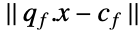
{qf, cf} = IconizedObject[«Block»];QuadraticOptimization[Norm[Inactive[Plus][qf.x, -cf]], VectorGreaterEqual[{x, 1}], x]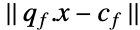
LeastSquares[qf, cf]濃度で制約された最小二乗問題. が最大で
 個の非零要素を持つように
 を最小化する:
m = 33; n = 7;k = 4;
SeedRandom[n * m * k];
a = RandomReal[{-1, 1}, {m, n}];
b = RandomReal[{-1, 1}, m]; が,もし
 ならば
 は非零となるような決定ベクトルであるとする.決定制約は次のようになる:
decisionConstraints = {Total[z] ≤ k, 0z1, z∈Vectors[n, Integers]}; のときの制約
 をモデル化するために,
 となるような大きい定数
 を選ぶ:
coeffConstraint = -100 zx100z;QuadraticOptimization[Norm[Inactive[Plus][a.x, -b]], {decisionConstraints, coeffConstraint}, {x, z}]部分集合の選択は,Fitで  正規化を使うとより効率よくできる.まず,最高で
 個の基底関数を使う正規化パラメータの範囲を求める:
nterms = Table[{λ, Length[Fit[{a, b},
	FitRegularization -> {"L1", λ}]["NonzeroPositions"]]}, {λ, 0.1, 2, 0.02}];
λk = Mean[MinMax[Cases[nterms, {x_, k} -> x]]]
fitTerms = Flatten[Fit[{a, b}, FitRegularization -> {"L1", λk}]["NonzeroPositions"]]Fit[{a[[All, fitTerms]], b}]関数集合候補から与えられたデータを近似する関数の最良の部分集合を求める:
refFun[x_] := Exp[-(5 * (x - 1 / 2)) ^ 2];
data = Table[{x, refFun[x]}, {x, 0, 1, 0.02}];
basis = Join[Cos[Range[10] * Pi * x], Sin[Range[10] * Pi * x]];
qf = DesignMatrix[data, basis, x, IncludeConstantBasis -> False];
cf = data[[All, 2]];functionConstraint = {Total[z] ≤ 5, 0z1};選択されなかった関数に関連付けられた係数は0でなければならない:
coeffConstraint = {-10 * zxz * 10};res = QuadraticOptimization[Inactive[Norm][Inactive[Plus][qf.x, -cf]] ^ 2, {functionConstraint, coeffConstraint}, {x,
z∈Vectors[Last[Dimensions[qf]], Integers]}]{coeffs, chosen} = {x, z} /. res;
fun = Total[Pick[basis * coeffs, chosen, 1]];
Plot[fun, {x, 0, 1}, Epilog -> Point[data], PlotRange -> All]分類問題 (2)



{set1, set2} = IconizedObject[«Block»];dataplot = ListPointPlot3D[{set1, set2}, Sequence[...]]分割するためには,集合1は 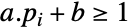 を,集合2は
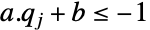 を満足しなければならない.
 を最小化することで超平面を求める:
res = QuadraticOptimization[Norm[a]^2, {set1.a + b1, set2.a + b-1}, {a, b}, Method -> "COIN"]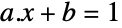


(2 / Norm[a]) /. resplane = (a.{x, y, z} + b) /. resShow[dataplot, ContourPlot3D[plane == 0, {x, -1, 1}, {y, -1, 1}, {z, -1, 1}, Sequence[...]]]

{set1, set2} = IconizedObject[«Block»];
dataplot = ListPointPlot3D[{set1, set2}, Sequence[...]]DesignMatrixを使って2つの集合についての二次多項式データ行列を構築する:
{data1, data2} = DesignMatrix[#, {x, x^2, y, y^2, x y}, {x, y}]& /@ {set1, set2};分割するためには,集合1は 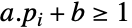 を,集合2は
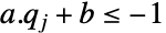 を満足しなければならない.
 を最小化することで分割曲面を求める:
res = QuadraticOptimization[Norm[a]^2, {data1.a + b1, data2.a + b-1}, {a, b}, Method -> "COIN"]poly = (a.{1, x, x^2, y, y^2, x y} + b) /. resShow[dataplot, ContourPlot3D[poly == 0, {x, -1.5, 1.5}, {y, -1.5, 1.5}, {z, -1, 1}, Sequence[...]]]幾何問題 (3)



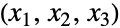
p0 = {1 / 2, -1, 1};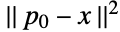 を最小化することで
 に最も近い点を求める.目的関数の構築にはInactive Plusを使う:
res = QuadraticOptimization[Norm[-p0 + x]^2, {{0, 0, 1}, {1, -2, 3}}.x == {0, 1}, x]Show[ContourPlot3D[{Subscript[x, 3] == 0, Subscript[x, 1] - 2Subscript[x, 2] + 3Subscript[x, 3] == 1}, {Subscript[x, 1], -1, 1}, {Subscript[x, 2], -1, 1}, {Subscript[x, 3], -1, 1}, Sequence[...]], IconizedObject[«Graphics3D»]]{region1, region2} = IconizedObject[«Block»];{dist, minPts} = QuadraticOptimization[Norm[x1 - x2] ^ 2, {x1∈region1, x2∈region2}, {x1, x2}, {"PrimalMinimumValue", "PrimalMinimizerRules"}]Show[region1, region2, Graphics3D[{Line[{x1, x2}], Blue, PointSize[0.025], Point[{x1, x2}]} /. minPts]]

region = [image];
pts = MeshCoordinates[region];
もとの最小化問題は, に従って
 を最小化するものである.この問題の双対は,
 に従って
 を最大化するものである:
obj = -Norm[w.pts]^2 + Total[pts^2, {2}].w;
constraints = {w0, Total[w] == 1};{weights, minval} = QuadraticOptimization[-obj, constraints, w∈Vectors[Length[pts]], {"PrimalMinimizer", "PrimalMinimumValue"}];
Short[weights, 3]
center = weights.pts包含している最小の球の半径は最大値のSqrtである:
radius = Sqrt[-minval]Show[Graphics3D[{Opacity[0.2], Red, Ball[center, radius]}], region]包含している最小の球はBoundingRegionを使って効率よく求めることができる:
BoundingRegion[pts, "MinBall"]投資問題 (3)
最低でも1000ドルの配当が得られリスクが最小となるように,資本金10000ドルを4つの株に割り当てる方法を求める.期待する戻り値と株式に関連付けられた共分散行列  は次の通りである:
{returnValue, R} = IconizedObject[«Block»];4つの株の単価は1ドルである.各株には最大で2500ドルを割り当てることができる:
capitalConstraint = x2500;returnConstraint = returnValue.x1000;minStock = x0;各株式に費やす金額の総量は, で与えられるリスクを最小化することで求められる:
res = QuadraticOptimization[x.R.x, {capitalConstraint,
returnConstraint, minStock}, x∈Vectors[4, Integers]]Total[x /. res]空売りオプションも含めて最低でも配当が1000ドルになるようにし,リスクが最小となるようにして,4つの株式から買う株の数を求める:
{returnValue, R} = IconizedObject[«Block»];資本金についての制約と投資に対する配当の制約は次の通りである:
constraints = {x2500, returnValue.x1000};空売りオプションを使用すると株が売却できる.目的関数  によって与えられるリスクを最小化することで,買う/空売りする株式の最適数がもとまる:
res = QuadraticOptimization[x.R.x, constraints, x∈Vectors[4, Integers]]2番目の株式は空売りすることができる.空売りで最低1000ドル得るための総投資額は以下の通りである:
Total[x /. res]空売りをしなければ,初期投資ははるかに大きくなければならない:
Total[x /. QuadraticOptimization[x.R.x, {constraints, x0}, x∈Vectors[4, Integers]]]リスクを最小限に抑えながら収益を最大化するために,可能性のある20の候補株の中から投資する6つの株の最適な組合せを求める:
{μ, Σ} = Block[...]; を株式
 で行われた総投資の割合とする.利益は
 で与えられる.ここで,
 は各株式の期待利益値のベクトルである:
return = μ.w; を決定ベクトルとし,
 の場合はその株を購入する.6つの銘柄を選択する必要がある:
decisionConstraints = {Total[x] == 6, 0x1};
weightConstraints = {0wx, Total[w] == 1}; で与えられるリスクを最小化して利益を最大化する最適な株式の組合せを求める:
res = QuadraticOptimization[w.Σ.w - return, {decisionConstraints,
weightConstraints}, {w, x∈Vectors[20, Integers]}, Tolerance -> 10 ^ -12];stockPicks = Flatten[Position[x /. res, 1]](w /. res)[[stockPicks]]ポートフォリオの最適化 (1)
リスクが最小で利益か最大になるような,資本の6つの株式への投資配分を求める:
{μ, Σ} = Block[...];株式  への投資の全投資に占める割合を
 としよう.利益は
 で与えられる.ただし,
 は個別の株式の予想収益の値のベクトルである:
return = μ.w;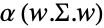

risk = w.Σ.w;目標は,指定されたリスク回避パラメータ  についてリスクを最小にしつつ利益を最大にすることである:
objective[α_ ? NumericQ] := -(return - α risk);投資  の割合はすべて0より大きく1に加えられなければならない:
weightConstraints = {w0, Total[w] == 1};リスク回避パラメータの範囲内で利益と対応するリスクを計算する:
frontier = Table[{risk, return} /. QuadraticOptimization[
	objective[α], weightConstraints, w], {α, Subdivide[0.0001, 3, 100]}];
範囲  における最適値
 は,リスクと利益のトレードオフにおける上包を与える:
randomRiskReturns = Table[{risk, return}, {w, Map[...]}];
Show[ListPlot[frontier, ...], ListPlot[randomRiskReturns, Rule[...]]]
指定された数のリスク回避パラメータについて投資  の占める割合を計算する:
riskAversionParameter = N@{1 / 100, 1 / 2, 1, 10, 100, 1000};
res = Table[{α, risk, w} /. QuadraticOptimization[
	objective[α], weightConstraints, w], {α, riskAversionParameter}];
リスク回避パラメータ  を大きくすると株式が多様化しリスクが軽減される:
Legended[BarChart[res[[All, -1]], ...], SwatchLegend[...]]リスク回避パラメータ  を大きくすると投資に対する予想収益が減少する:
ListLogLogPlot[Transpose[{res[[All, 1]], res[[All, -1]].μ}], ...]軌道最適化問題 (2)
 に従って
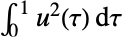 を最小化する.最小化関数積分は台形規則を使って近似することができる.離散化された目的関数は
 である:
{ti, wts} = Most[IconizedObject[«NIntegrate`TrapezoidalRuleData»]];
W = DiagonalMatrix[SparseArray[wts]];
obj = u.W.u;
mat = IconizedObject[«NDSolve`FiniteDifferenceDerivative[2, ti, DifferenceOrder -> 2]»];
ode = mat.x == u;
制約条件  はIndexed関数を使って表すことができる:
bc1 = {Indexed[x, 1] == 0, Indexed[x, Length[ti]] == 1};制約条件  は有限差分を使って離散化することができる.最初と最後の行だけが使われる:
mat = IconizedObject[«NDSolve`FiniteDifferenceDerivative[1, ti, DifferenceOrder -> 2]»];
bc2 = mat[[{1, -1}]].x == 0;res = QuadraticOptimization[obj, {ode, bc1, bc2}, {u, x}];
Short[res, 6]離散化された結果をInterpolatingFunctionに変換する:
{xsol, usol} = ListInterpolation[#, ti]& /@ ({x, u} /. res);Row[{Plot[{xsol[t], 3t^2 - 2t^3}, {t, 0, 1}, Sequence[...]], Plot[{usol[t], 6 - 12t}, {t, 0, 1}, Sequence[...]]}]2点間の最短経路を障害物を避けながら求める.障害物を指定する:
SeedRandom[1234];mesh = ConvexHullMesh[RandomReal[{.2, .8}, {10, 2}]];{a, b} = LinearOptimization[0, {}, Element[x, mesh], "LinearInequalityConstraints"];start = {0, 0};
end = {1, 1};この経路は  点を使って離散化できる.
 が位置ベクトルを表すとする:
n = 10;
pvars = Table[Element[p[i], Vectors[2, Reals]], {i, 1, n}];
目的は を最小化することである.
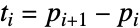 とする.目的は
 に変換された:
tvars = Table[t[i], {i, n - 1}];
transformationConstraint = Table[t[i] == p[i + 1] - p[i], {i, n - 1}];
objective = Sum[t[i].t[i], {i, n - 1}];endPointConstraints = {p[1] == start, p[n] == end};maxDist = 2 Norm[start - end] / n;
separationConstraints = Table[-maxDist t[i]maxDist ,
{i, n - 1}]; の要素の少なくとも1つが0未満のとき,点
 は目的の外になる.この制約条件を強制するために,
 が決定ベクトルで
 が
 となるような
 の

 番目の要素であるとする.こうすると
 となり
 は
 となるための十分大きくなる:
m = 10;
zvars = Table[Element[z[i], Vectors[Length[a], Integers]], {i, n}];
binaryConstraints = Table[0 z[i] 1, {i, n}];
avoidanceConstraints = Table[{Inactive[Plus][a.p[i], b] m z[i], Total[z[i]] ≤ Length[a] - 1}, {i, n}];res = QuadraticOptimization[objective, {endPointConstraints, transformationConstraint, separationConstraints, binaryConstraints, avoidanceConstraints}, Join[pvars, tvars, zvars]];path = Table[p[i], {i, n}] /. res;
Show[mesh, Graphics[{Point[path], Line[path]}]]障害物との潜在的な交差を避けるために,領域を膨張させて問題をもう一度解く:
newMesh = RegionResize[mesh, {Scaled[1.45], Scaled[1.45]}];
{a, b} = LinearOptimization[0, {}, Element[x, newMesh], "LinearInequalityConstraints"];avoidanceConstraints = Table[{Inactive[Plus][a.p[i], b] m z[i],
Total[z[i]] ≤ Length[a] - 1}, {i, n}];res = QuadraticOptimization[objective, {endPointConstraints, transformationConstraint, separationConstraints, binaryConstraints, avoidanceConstraints}, Join[pvars, tvars, zvars]];path = Table[p[i], {i, n}] /. res;
Show[ mesh, Graphics[{Point[path], Line[path]}]]最適制御問題 (2)



A = (| | |
| --- | --- |
| -1 | 0.5 |
| 0.3 | -1 |);{ti, wts} = 10 * Most[IconizedObject[«NIntegrate`TrapezoidalRuleData»]];
W = DiagonalMatrix[SparseArray[wts]];
objective = x1.W.x1 + s.W.s + u.W.u;
auxConstraint = s == (1 - x2);
dTMat = IconizedObject[«NDSolve`FiniteDifferenceDerivative[1, ti, DifferenceOrder -> 2]»];
ode1 = dTMat.x1 == A[[1]].{x1, x2} + u;
ode2 = dTMat.x2 == A[[2]].{x1, x2} + u;
端末条件の制約  はIndexedを使って指定できる:
bc1 = {Indexed[x1, 1] == 1, Indexed[x2, 1] == 0};
bc2 = { Indexed[x1, Length[ti]] == 0, Indexed[x2, Length[ti]] == 1};res = QuadraticOptimization[objective, {ode1, ode2, bc1, bc2, auxConstraint}, {u, x1, x2, s}];離散化された結果をInterpolatingFunctionに変換する:
{usol, x1sol, x2sol} = Map[ListInterpolation[#, ti]&, {u, x1, x2} /. res];Plot[usol[t], {t, 0, 10}]Plot[{x1sol[t], x2sol[t]}, {t, 0, 10}]



A = (| | |
| --- | --- |
| -1 | 0.5 |
| 0.3 | -1 |);{ti, wts} = 10 * Most[IconizedObject[«NIntegrate`TrapezoidalRuleData»]];
W = DiagonalMatrix[SparseArray[wts]];
objective = g.W.g + s.W.s + u.W.u;
auxConstraint1 = g == (1 / 2 - x1);
auxConstraint2 = s == (1 - x2);
dTMat = IconizedObject[«NDSolve`FiniteDifferenceDerivative[1, ti, DifferenceOrder -> 2]»];
ode1 = dTMat.x1 == A[[1]].{x1, x2} + u;
ode2 = dTMat.x2 == A[[2]].{x1, x2} + u;
端末条件の制約  はIndexedを使って指定できる:
bc1 = {Indexed[x1, 1] == 1, Indexed[x2, 1] == 0};
bc2 = { Indexed[x1, Length[ti]] == 1 / 2, Indexed[x2, Length[ti]] == 1};
controlConstraint = {u-10, u5};res = QuadraticOptimization[objective, {ode1, ode2, bc1, bc2, auxConstraint1, auxConstraint2, controlConstraint}, {u, x1, x2, s, g}];離散化された結果をInterpolatingFunctionに変換する:
{usol, x1sol, x2sol} = Map[ListInterpolation[#, ti]&, {u, x1, x2} /. res];
Plot[usol[t], {t, 0, 10}, PlotRange -> All]Plot[{x1sol[t], x2sol[t]}, {t, 0, 10}]逐次二次最適化 (2)
非線形制約条件  に従って非線形関数
 を最小化する.最小化は,
 を
 として,また制約条件
 を
 として近似することで行える.こうすると,反復的に解ける二次最小化問題になる.
 で
 である場合について考える:
f[{x_, y_}] := 1 - Exp[-(Sin[x] ^ 2 + Sin[y - 1 / 2] ^ 2)];
g[{x_, y_}] := {-x + 0.5, y + 0.5, x - y + 1};df[{x_, y_}] = D[f[{x, y}], {{x, y}}];
hf[{x_, y_}] = D[f[{x, y}], {{x, y}, 2}];dg[{x_, y_}] = D[g[{x, y}], {{x, y}}];下位問題は, に従って
 を最小化することで
 を求めることである:
QuadraticSubProblem[xiter_] := Module[{q, c, a, b, res},
	{q, c, a, b} = #[xiter]& /@ {hf, df, dg, g};
	res = Quiet[QuadraticOptimization[{q, c}, {a, b}]];
	If[!VectorQ[res, NumericQ], res = LinearOptimization[c, {a, b}];
	];
	res
	];
最初の推測  から始めて反復する.次の反復は
 である.ただし,
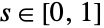 は制約条件が常に満足されるためのステップ長である:
x^ *  = {-1, -0.4};
xp = Last@Reap[Do[
	Sow[x^ * , "IterationPoints"];
	d = QuadraticSubProblem[x^ * ];
	If[Norm[d] ≤ 10 ^ -8, Break[]];
	s = 1;
	While[Min[g[x^ *  + s * d]] ≤ 0, s /= 2];
	x^ *  += s * d;
, {20}], "IterationPoints"]ContourPlot[f[{x, y}], {x, -1.5, 0.5}, {y, -0.5, 1.5}, Sequence[...]]

f[{x_, y_}] := Sqrt[(1 + x ^ 2 + Cos[y / 2] ^ 2)];
g[{x_, y_}] := {x + Sin[2y] - 1, -y + 2};
gEq[{x_, y_}] := {x y - 2};df[{x_, y_}] = D[f[{x, y}], {{x, y}}];
hf[{x_, y_}] = D[f[{x, y}], {{x, y}, 2}];dg[{x_, y_}] = D[g[{x, y}], {{x, y}}];
dgEq[{x_, y_}] = D[gEq[{x, y}], {{x, y}}];


QuadraticSubProblem[xiter_] := Module[{q, c, a, b, aeq, beq, res},
	{q, c, a, b, aeq, beq} = #[xiter]& /@ {hf, df, dg, g, dgEq, gEq};
	res = Quiet[QuadraticOptimization[{q, c}, {a, b}, {aeq, beq}]];
	If[!VectorQ[res, NumericQ], res = LinearOptimization[c, {a, b}, {aeq, beq}];
	];
	res
	];
x^ *  = {0.5, 0.5};
xp = Last@Reap[Do[
	Sow[x^ * , "IterationPoints"];
	d = QuadraticSubProblem[x^ * ];
	If[Norm[d] ≤ 10 ^ -8, Break[]];
	s = 1;
	While[Min[g[x^ *  + s * d]] ≤ 0 && s > 10 ^ -9, s /= 2];
	x^ *  += s * d;
, {30}], "IterationPoints"]ContourPlot[f[{x, y}], {x, 0, 2.5}, {y, 0, 2}, ...]特性と関係 (9)
QuadraticOptimizationは目的関数の大域的最小値を与える:
{Subscript[x, min], minval} = QuadraticOptimization[x^2 + y^2 - 2x - 6y, {x + 2y ≥ 4, x ≤ 3}, {x, y}, {"PrimalMinimizer", "PrimalMinimumValue"}]Show[Plot3D[x^2 + y^2 - 2x - 6y, ...], Graphics3D[{Blue, PointSize[0.05], Point[Append[Subscript[x, min], minval]]}]]Table[{Subscript[x, min], minval} = QuadraticOptimization[x^2 + y^2 + c.{x, y}, ...];
Show[...], {c, {{-2, -6}, {-10, -6}, {-10, 6}}}]Minimizeは二次最適化問題の大域的厳密結果を与える:
Minimize[{2x^2 + 20y^2 + 6x y + 5x, {-x + y ≥ 2, y ≥ 0}}, {x, y}]NMinimizeを使って,大域法を使った近似結果を得ることができる:
NMinimize[{2x^2 + 20y^2 + 6x y + 5x, {-x + y ≥ 2, y ≥ 0}}, {x, y}]FindMinimumを使って局所法を使った近似結果を得ることができる:
FindMinimum[{2x^2 + 20y^2 + 6x y + 5x, {-x + y ≥ 2, y ≥ 0}}, {x, y}]LinearOptimizationはQuadraticOptimizationの特殊ケースである:
QuadraticOptimization[x + 2y, {3x + 4y ≥ 5 && x ≥ 0 && y ≥ 0}, {x, y}]LinearOptimization[x + 2y, {3x + 4y ≥ 5 && x ≥ 0 && y ≥ 0}, {x, y}]//NQuadraticOptimization[{0, {1, 2}}, {{{3, 4}, {1, 0}, {0, 1}}, {-5, 0, 0}}]SecondOrderConeOptimizationはQuadraticOptimizationの一般化である:
obj = 2x^2 + 20y^2 + 6x y + 5x;
cons = {-x + y ≥ 2, y ≥ 0};QuadraticOptimization[obj, cons, {x, y}]


SecondOrderConeOptimization[t, {obj ≤ t, cons}, {x, y, t}]SemidefiniteOptimizationはQuadraticOptimizationの一般化である:
obj = 2x^2 + 20y^2 + 6x y + 5x;
cons = {-x + y ≥ 2, y ≥ 0};QuadraticOptimization[obj, cons, {x, y}]


SemidefiniteOptimization[t, {obj ≤ t, cons}, {x, y, t}]ConicOptimizationはQuadraticOptimizationの一般化である:
obj = 2x^2 + 20y^2 + 6x y + 5x;
cons = {-x + y ≥ 2, y ≥ 0};QuadraticOptimization[obj, cons, {x, y}]


ConicOptimization[t, {obj ≤ t, cons}, {x, y, t}]考えられる問題 (6)
狭義の不等式を使って指定された制約条件は,メソッドによっては満足されないかもしれない:
{obj, cons} = {x ^ 2 + x + y, {x - 2y ≤ 3, x > 1, y > 0}};理由は,QuadraticOptimizationを解くと  になるからである:
cons /. QuadraticOptimization[obj, cons, {x, y}, Method -> "CSDP"]
QuadraticOptimization[x ^ 2, {x ≤ 0, x ≥ 1}, x, "PrimalMinimumValue"]
ミニマイザは Indeterminateである:
QuadraticOptimization[x ^ 2, {x ≤ 0, x ≥ 1}, x]

QuadraticOptimization[x ^ 2 + y, 0 ≤ x ≤ 1, {x, y}, "PrimalMinimumValue", Method -> "CSDP"]
ミニマイザはIndeterminateである:
QuadraticOptimization[x ^ 2 + y, 0 ≤ x ≤ 1, {x, y}, Method -> "CSDP"]
obj = (x - 1)^2 + (y - 5 / 2)^2;
cons = x + 2y ≤ 4;QuadraticOptimization[obj, cons, {x, y}, "FactoredObjectiveMatrix"]QuadraticOptimization[obj, cons, {x, y}, "FactoredObjectiveVector"]混合整数問題に対する双対に関連した解の特性は得られないかもしれない:
QuadraticOptimization[2x^2 + 20y^2 + 6x y + 5x, -x + y ≥ 2, {x∈Integers, y∈Reals}, {"DualMaximumValue", "DualMaximizer", "DualityGap"}]複素数値を含む制約条件はベクトル不等式で指定しなければならない:
QuadraticOptimization[Inactive[Norm][{x}] ^ 2, {xI}, {x∈Complexes}]GreaterEqualを使うだけではうまくいかない:
QuadraticOptimization[Inactive[Norm][{x}] ^ 2, {x ≥ I}, {x∈Complexes}]

テキスト
Wolfram Research (2019), QuadraticOptimization, Wolfram言語関数, https://reference.wolfram.com/language/ref/QuadraticOptimization.html (2020年に更新).
CMS
Wolfram Language. 2019. "QuadraticOptimization." Wolfram Language & System Documentation Center. Wolfram Research. Last Modified 2020. https://reference.wolfram.com/language/ref/QuadraticOptimization.html.
APA
Wolfram Language. (2019). QuadraticOptimization. Wolfram Language & System Documentation Center. Retrieved from https://reference.wolfram.com/language/ref/QuadraticOptimization.html