SecondOrderConeOptimization[c,{{a1,b1,α1,β1},…,{ak,bk,αk,βk}}]
finds a vector ![]() that minimizes
that minimizes ![]() subject to the constraints
subject to the constraints ![]() .
.
SecondOrderConeOptimization[c,…,{dom1,dom2,…}]
takes ![]() to be in the domain domi, where domi is Integers or Reals.
to be in the domain domi, where domi is Integers or Reals.


SecondOrderConeOptimization
SecondOrderConeOptimization[f,cons,vars]
finds values of variables vars that minimize the linear objective f subject to second-order cone and/or linear constraints cons.
SecondOrderConeOptimization[c,{{a1,b1,α1,β1},…,{ak,bk,αk,βk}}]
finds a vector ![]() that minimizes
that minimizes ![]() subject to the constraints
subject to the constraints ![]() .
.
SecondOrderConeOptimization[c,…,{dom1,dom2,…}]
takes ![]() to be in the domain domi, where domi is Integers or Reals.
to be in the domain domi, where domi is Integers or Reals.
SecondOrderConeOptimization[…,"prop"]
specifies what solution property "prop" should be returned.
Details and Options
- Second-order cone optimization is also known as second-order cone programming (SOCP) and mixed-integer second-order cone programming (MISOCP).
- Second-order cone optimization is used in problems such as parameter fitting and geometric distance problems.
- Second-order cone optimization is a convex optimization problem that can be solved globally and efficiently with real, integer or complex variables.
- Second-order cone optimization finds
 that solves the primal problem:
 -
minimize 
subject to constraints ![TemplateBox[{{{{a, _, i}, ., x}, +, {b, _, i}}}, Norm]<=alpha_i.x+beta_i, i=1,..., k](Files/SecondOrderConeOptimization.en/7.png "TemplateBox[{{{{a, _, i}, ., x}, +, {b, _, i}}}, Norm]<=alpha_i.x+beta_i, i=1,..., k")
where 
- Mixed-integer second-order cone optimization finds
 and
and  that solve the problem:
 -
minimize 
subject to constraints ![TemplateBox[{{{{a, _, {(, {j, _, r}, )}}, ., x}, +, {{a, _, {(, {j, _, r}, )}}, ., {yb, _, j}}}}, Norm]<=alpha_(j_r).x+alpha_(j_i).y+beta_j, j=1,..., k](Files/SecondOrderConeOptimization.en/12.png "TemplateBox[{{{{a, _, {(, {j, _, r}, )}}, ., x}, +, {{a, _, {(, {j, _, r}, )}}, ., {yb, _, j}}}}, Norm]<=alpha_(j_r).x+alpha_(j_i).y+beta_j, j=1,..., k")
where 
- When the objective function is real valued, SecondOrderConeOptimization solves problems with
![x in TemplateBox[{}, Complexes]^n](Files/SecondOrderConeOptimization.en/14.png "x in TemplateBox[{}, Complexes]^n") by internally converting to real variables
by internally converting to real variables  , where
  and
and  .
. - The variable specification vars should be a list with elements giving variables in one of the following forms:
-
v variable with name  and dimensions inferred
v∈Reals real scalar variable v∈Integers integer scalar variable v∈Complexes complex scalar variable v∈ℛ vector variable restricted to the geometric region 
v∈Vectors[n,dom] vector variable in  or
or 
v∈Matrices[{m,n},dom] matrix variable in  or
or 
- Note that linear constraints may be expressed using second-order constraints. For convenience, a single 0 is interpreted as needed as a matrix or vector with zero entries:
-
{ai,bi,0,0} linear equality constraints 
{0,0,αi,βi} linear inequality constraint 
- The constraints cons can be specified by:
-
LessEqual 
scalar inequality GreaterEqual 
scalar inequality VectorLessEqual 
vector inequality VectorGreaterEqual 
vector inequality Equal 
scalar or vector equality Element 
convex domain or region element - With SecondOrderConeOptimization[f,cons,vars], parameter equations of the form parval, where par is not in vars and val is numerical or an array with numerical values, may be included in the constraints to define parameters used in f or cons.
- The primal minimization problem has a related maximization problem that is the Lagrangian dual problem. The dual maximum value is always less than or equal to the primal minimum value, so it provides a lower bound. The dual maximizer provides information about the primal problem, including sensitivity of the minimum value to changes in the constraints.
- The second-order cone optimization has a dual: » »
-
maximize 
subject to constraints ![sum_(i=1)^k(a_i.y_i+alpha_ilambda_i)⩵c, ; TemplateBox[{{y, _, i}}, Norm]<=lambda_i, i=1,..., k](Files/SecondOrderConeOptimization.en/34.png "sum_(i=1)^k(a_i.y_i+alpha_ilambda_i)⩵c, ; TemplateBox[{{y, _, i}}, Norm]<=lambda_i, i=1,..., k")
where 
- For second-order cone optimization, strong duality always holds, meaning that if there is a solution to the primal minimization problem, then there is a solution to the dual maximization problem, and the dual maximum value is equal to the primal minimum value.
- The possible solution properties "prop" include:
-
"PrimalMinimizer" 
a list of variable values that minimizes the objective function "PrimalMinimizerRules" 
values for the variables vars={v1,…} that minimize 
"PrimalMinimizerVector" 
the vector that minimizes 
"PrimalMinimumValue" 
the minimum value 
"DualMaximizer" 
the maximizing dual vector "DualMaximumValue" 
the dual maximizing value "DualityGap" 
the difference between the dual and primal optimal values "Slack" 
vector that converts inequality constraints to equality "ConstraintSensitivity" 
sensitivity of  to constraint perturbations
"ObjectiveVector" 
the linear objective vector "SecondOrderConeConstraints" 
the list of coefficients for the constraints "LinearEqualityConstraints" 
the linear equality constraint matrix and vector {"prop1","prop2",…} several solution properties - The following options may be given:
-
MaxIterations Automatic maximum number of iterations to use Method Automatic the method to use PerformanceGoal $PerformanceGoal aspects of performance to try to optimize Tolerance Automatic the tolerance to use for internal comparisons - The option Method->method may be used to specify the method to use. Available methods include:
-
Automatic choose the method automatically "SCS" SCS splitting conic solver "CSDP" CSDP semidefinite optimization solver "DSDP" DSDP semidefinite optimization solver "PolyhedralApproximation" approximate constraints using polyhedra "MOSEK" commercial MOSEK convex optimization solver "Gurobi" commercial Gurobi linear and quadratic optimization solver "Xpress" commercial Xpress linear and quadratic optimization solver - Computations are limited to MachinePrecision.
Examples
open all close allBasic Examples (4)
Minimize ![]() subject to the constraint
subject to the constraint ![]() :
:
res = SecondOrderConeOptimization[x + y, Norm[{x, y}] ≤ 1, {x, y}]The optimal point lies in a region defined by the constraints and where ![]() is smallest within the region:
is smallest within the region:
Show[Plot3D[x + y, {x, -1, 1}, {y, -1, 1}, ...], Graphics3D[{Blue, PointSize[0.05], Point[{x, y, x + y} /. res]}]]Minimize ![]() subject to the constraints
subject to the constraints ![]() :
:
res = SecondOrderConeOptimization[x + y, {x^2 + y^2 ≤ 1, (x - 1 / 2)^2 + y^2 ≤ 1}, {x, y}]The optimal point lies on the smallest value of ![]() in a region bounded by the intersection of two disks:
in a region bounded by the intersection of two disks:
ContourPlot[x + y, {x, y}∈ImplicitRegion[x^2 + y^2 ≤ 1 && (x - 1 / 2)^2 + y^2 ≤ 1,
	{x, y}], Contours -> 10, ...]
Minimize ![]() subject to the constraints
subject to the constraints ![]() . Specify the inputs in matrix-vector form:
. Specify the inputs in matrix-vector form:
c = {1, 1, 0};
con1 = {{{1, 0, 0}, {0, 1, 0}, {0, 0, 0}}, 0, 0, 1};
con2 = {{{0, 0, 0}, {0, 1, 0}, {0, 0, 1}}, 0, 0, 1};
con3 = {{{-1, 0, 1}}, {1 / 2}, 0, 0};
Solve the problem using matrix-vector form:
SecondOrderConeOptimization[c, {con1, con2, con3}]Minimize ![]() subject to the constraint
subject to the constraint ![]() :
:
SecondOrderConeOptimization[x + y, Norm[{x, y}] ≤ 1, {x∈Integers, y∈Reals}]Use the equivalent matrix-vector form:
c = {1, 1};
{a1, b1, α1, β1} = {{{1, 0}, {0, 1}}, {0, 0}, {0, 0}, 1};
SecondOrderConeOptimization[c, {{a1, b1, α1, β1}}, {Integers, Reals}]
Scope (27)
Basic Uses (9)
Minimize ![]() subject to the constraints
subject to the constraints ![]() :
:
SecondOrderConeOptimization[x + y, {Norm[{x, y}] ≤ 1, y ≥ 0}, {x, y}]Get the minimizing value using solution property "PrimalMinimiumValue":
SecondOrderConeOptimization[x + y, {Norm[{x, y}] ≤ 1, y ≥ 0}, {x, y}, "PrimalMinimumValue"]Minimize ![]() subject to the constraints
subject to the constraints ![]() :
:
SecondOrderConeOptimization[x + y, {x^2 + y^2 ≤ 1, y ≥ 0}, {x, y}]Get the minimizing value and minimizing vector using solution properties:
SecondOrderConeOptimization[x + y, {x^2 + y^2 ≤ 1, y ≥ 0}, {x, y}, {"PrimalMinimumValue", "PrimalMinimizer"}]Minimize ![]() subject to the constraints
subject to the constraints ![]() :
:
SecondOrderConeOptimization[x + y, {Norm[{x, y}] ≤ 1, y ≥ 0}, {x, y}]Define the objective as ![]() and the constraints as
and the constraints as ![]() :
:
c = {1, 1};
{Subscript[a, 1], Subscript[b, 1], Subscript[α, 1], Subscript[β, 1]} = {{{1, 0}, {0, 1}}, 0, 0, 1};
{Subscript[a, 2], Subscript[b, 2], Subscript[α, 2], Subscript[β, 2]} = {0, 0, {0, 1}, 0};
Solve using matrix-vector inputs:
SecondOrderConeOptimization[c, {{Subscript[a, 1], Subscript[b, 1], Subscript[α, 1], Subscript[β, 1]}, {Subscript[a, 2], Subscript[b, 2], Subscript[α, 2], Subscript[β, 2]}}]Minimize ![]() subject to the constraints
subject to the constraints ![]() :
:
SecondOrderConeOptimization[x + y, {Norm[{x, y}] ≤ 1, x + y == 1 / 2, y ≥ 0}, {x, y}]Define the objective as ![]() and the constraints as
and the constraints as ![]() :
:
c = {1, 1};
{Subscript[a, 1], Subscript[b, 1], Subscript[α, 1], Subscript[β, 1]} = {{{1, 0}, {0, 1}}, 0, 0, 1};
{Subscript[a, 2], Subscript[b, 2], Subscript[α, 2], Subscript[β, 2]} = {0, 0, {0, 1}, 0};
Specify the equality constraint as:
{Subscript[a, 3], Subscript[b, 3], Subscript[α, 3], Subscript[β, 3]} = {{{1, 1}}, {-1 / 2}, 0, 0};Solve using matrix-vector inputs:
SecondOrderConeOptimization[c, {{Subscript[a, 1], Subscript[b, 1], Subscript[α, 1], Subscript[β, 1]}, {Subscript[a, 2], Subscript[b, 2], Subscript[α, 2], Subscript[β, 2]},
	{Subscript[a, 3], Subscript[b, 3], Subscript[α, 3], Subscript[β, 3]}}]
Minimize ![]() subject to the constraint
subject to the constraint ![]() using constant parameter equations for a and b:
using constant parameter equations for a and b:
peqns = {a == {{1, 2}, {3, 4}, {5, 6}}, b == {1, 1, 1}};SecondOrderConeOptimization[t, {peqns, Norm[a.{x, y} + b] ≤ t}, {x, y, t}]Minimize ![]() subject to the constraint
subject to the constraint ![]() using vector variable
using vector variable ![]() :
:
peqns = {a == {{1, 2}, {3, 4}, {5, 6}}, b == {1, 1, 1}};SecondOrderConeOptimization[t, {peqns, Norm[a.x + b] ≤ t}, {x, t}]Minimize ![]() subject to the constraint
subject to the constraint ![]() :
:
SecondOrderConeOptimization[t, {a == {{1, 2}, {3, 4}, {5, 6}}, b == {1, 1, 1}, Norm[a.{x, y} + b] ≤ t, -1 ≤ x ≤ 1, -1 ≤ y ≤ 1}, {x, y, t}]Specify the constraints using VectorGreaterEqual () and VectorLessEqual ():
SecondOrderConeOptimization[t, {a == {{1, 2}, {3, 4}, {5, 6}}, b == {1, 1, 1}, Norm[a.{x, y} + b] ≤ t, {-1, -1}{x, y}{1, 1}}, {x, y, t}]Minimize ![]() subject to
subject to ![]() . Use Inactive[Plus] to avoid unintentional threading:
. Use Inactive[Plus] to avoid unintentional threading:
{a, b} = {{{1, 2}, {3, 4}, {5, 6}}, {1, 1, 1}};
SecondOrderConeOptimization[t, Norm[a.v + b] ≤ t, {v, t}]
Specify the matrix ![]() and vector
and vector ![]() as parametrized equations to avoid using Inactive:
as parametrized equations to avoid using Inactive:
SecondOrderConeOptimization[t, {a1 == a, b1 == b, Norm[a1.v + b1] ≤ t}, {v, t}]Minimize ![]() subject to
subject to ![]() . Use NonNegativeReals to specify constraint
. Use NonNegativeReals to specify constraint ![]() :
:
SecondOrderConeOptimization[t, {a == {{1, 2}, {3, 4}, {5, 6}}, b == {1, 1, 1}, Norm[a.x + b] ≤ t, x - 1 == s}, {x, t, s∈Vectors[2, NonNegativeReals]}]Integer Variables (4)
Specify integer domain constraints using Integers:
SecondOrderConeOptimization[x + y, {Norm[{x, y}] ≤ 1, y ≥ 1 / 4}, {x∈Integers, y∈Integers}]Specify integer domain constraints on vector variables using Vectors[n,Integers]:
SecondOrderConeOptimization[Total[x], {Norm[x] ≤ 1, Indexed[x, 2] ≥ 1 / 4}, x∈Vectors[2, Integers]]Specify non-negative integer domain constraints using NonNegativeIntegers (![]() ):
):
SecondOrderConeOptimization[Total[x], {Norm[x] ≤ 3}, x∈Vectors[2, NonNegativeIntegers]]Specify non-positive integer domain constraints using NonPositiveIntegers (![]() ):
):
SecondOrderConeOptimization[Total[x], {Norm[x] ≤ 3}, x∈Vectors[2, NonPositiveIntegers]]Complex Variables (4)
Specify complex variables using Complexes:
SecondOrderConeOptimization[Re[z] + Im[z], zI, z∈Complexes]Use Abs[z] with complex z in the constraints:
SecondOrderConeOptimization[Re[z] + Im[z], Abs[z] ≤ 2, z∈ Complexes]SecondOrderConeOptimization[x + y, Norm[{x, y}] ≤ 2, {x, y}]Use a quadratic constraint ![]() with Hermitian matrix
with Hermitian matrix ![]() and real-valued variables:
and real-valued variables:
{q, c} = {{{2, 1 + I}, {1 - I, 1}}, {2, 3}};
SecondOrderConeOptimization[{1, 2}.x, (1 / 2) * x.q.x + c.x1, x∈Vectors[2, Reals]]Use constraint ![]() with a Hermitian matrix
with a Hermitian matrix ![]() and complex variables:
and complex variables:
q = {{3, 1 + I}, {1 - I, 2}};
SecondOrderConeOptimization[{1, 2}.Re[x], {(1 / 2) * Inactive[Dot][Conjugate[x], q, x]5}, x∈Vectors[2, Complexes]]Primal Model Properties (3)
Minimize ![]() subject to the constraints
subject to the constraints ![]() :
:
SecondOrderConeOptimization[x + y, {x^2 + y^2 ≤ 1, y ≥ 0}, {x, y}]Get the primal minimizer as a vector:
SecondOrderConeOptimization[x + y, {x^2 + y^2 ≤ 1, y ≥ 0}, {x, y}, "PrimalMinimizer"]SecondOrderConeOptimization[x + y, {x^2 + y^2 ≤ 1, y ≥ 0}, {x, y}, "PrimalMinimumValue"]Obtain the primal minimum value using symbolic inputs:
obj = x + y + 1;
cons = {x^2 + y^2 ≤ 1, y ≥ 0};Subscript[p, sym] = SecondOrderConeOptimization[obj, cons, {x, y}, "PrimalMinimumValue"]Extract the matrix-vector inputs of the optimization problem:
{c, socCons} = SecondOrderConeOptimization[obj, cons, {x, y}, {"ObjectiveVector", "SecondOrderConeConstraints"}];Solve using matrix-vector form:
Subscript[p, m] = SecondOrderConeOptimization[c, socCons, "PrimalMinimumValue"]Recover the symbolic primal value by adding the objective constant:
const = SecondOrderConeOptimization[obj, cons, {x, y}, "ObjectiveConstant"]Subscript[p, sym] == Subscript[p, m] + constFind the slack ![]() associated with a minimization problem:
associated with a minimization problem:
obj = x + y;
cons = {x^2 + y^2 ≤ 1, y ≥ 0, x + y == 1 / 2};s = SecondOrderConeOptimization[obj, cons, {x, y}, "Slack"]Get the primal minimum value ![]() and the constraints:
and the constraints:
{x^ * , socCons} = SecondOrderConeOptimization[obj, cons, {x, y}, {"PrimalMinimizer", "SecondOrderConeConstraints"}];The slack for constraint ![]() is a scalar
is a scalar ![]() such that
such that ![]() :
:
Table[{a, b, α, β} = socCons[[i]];
	If[α === 0, 0, α.x^ * ] + β - If[a === 0, 0, Norm[a.x^ *  + b]], {i, 3}] == s
Dual Model Properties (3)
c = {1, 1};
{Subscript[a, 1], Subscript[b, 1], Subscript[α, 1], Subscript[β, 1]} = {{{1, 0}, {0, 1}}, {0, 0}, {0, 0}, 1};
{Subscript[a, 2], Subscript[b, 2], Subscript[α, 2], Subscript[β, 2]} = {{{1, 0}, {0, 0}}, {-1 / 2, 0}, {0, 0}, 0};
xv = Table[Indexed[x, i], {i, 2}];psol = SecondOrderConeOptimization[c.xv, {Norm[Subscript[a, 1].xv + Subscript[b, 1]] ≤ Subscript[α, 1].xv + Subscript[β, 1],
Norm[Subscript[a, 2].xv + Subscript[b, 2]] ≤ Subscript[α, 2].xv + Subscript[β, 2]}, xv]The dual problem is to maximize ![]() subject to
subject to ![]() and
and ![]() :
:
{yv, λv} = {{y1, y2}, Table[Indexed[λ, i], {i, 2}]};dobj = Sum[(Subscript[b, i].yv[[i]] + Subscript[β, i]λv[[i]]), {i, 2}];dcon1 = Sum[(Subscript[a, i].yv[[i]] + Subscript[α, i]λv[[i]]), {i, 2}] == c;
dcon2 = Table[Norm[yv[[i]]] ≤ λv[[i]], {i, 2}];Solve the resulting maximization problem:
dsol = SecondOrderConeOptimization[dobj, {dcon1, dcon2}, Join[yv, λv]]The primal minimum value and the dual maximum value coincide because of strong duality:
{c.xv /. psol, -dobj /. dsol}That is the same as having a duality gap of zero. In general ![]() :
:
SecondOrderConeOptimization[c.xv, {Norm[Subscript[a, 1].xv + Subscript[b, 1]] ≤ Subscript[α, 1].xv + Subscript[β, 1],
	Norm[Subscript[a, 2].xv + Subscript[b, 2]] ≤ Subscript[α, 2].xv + Subscript[β, 2]}, xv, "DualityGap"]
Construct the dual problem using constraint matrices extracted from the primal problem:
{c, socCons} = SecondOrderConeOptimization[x + y, {x ^ 2 + y ^ 2 ≤ 1, x == 1 / 2}, {x, y}, {"ObjectiveVector", "SecondOrderConeConstraints"}];The dual problem is to maximize ![]() subject to
subject to ![]() and
and ![]() :
:
{yv, λv} = {{y1, y2}, Table[Indexed[λ, i], {i, 2}]};
{a, b, α, β} = Transpose[socCons];dobj = Sum[(If[b[[i]] === 0, 0, b[[i]].yv[[i]]] + β[[i]]λv[[i]]), {i, 2}];dcon1 = Sum[If[a[[i]] === 0, 0, a[[i]].yv[[i]]] + α[[i]]λv[[i]], {i, 2}] == c;
dcon2 = Table[Norm[yv[[i]]] ≤ λv[[i]], {i, 2}];Solve the resulting maximization problem:
dsol = SecondOrderConeOptimization[dobj, {dcon1, dcon2}, Join[yv, λv]]Get the dual maximum value directly using solution properties:
SecondOrderConeOptimization[x + y, {x ^ 2 + y ^ 2 ≤ 1, y ≥ 0, x ≤ -1 / 2}, {x, y}, "DualMaximumValue"]Get the dual maximizer directly using solution properties:
SecondOrderConeOptimization[x + y, {x ^ 2 + y ^ 2 ≤ 1, y ≥ 0, x ≤ -1 / 2}, {x, y}, "DualMaximizer"]Sensitivity Properties (4)
Use "ConstraintSensitivity" to find the change in optimal value due to constraint relaxations:
{c, {Subscript[a, 1], Subscript[b, 1], Subscript[α, 1], Subscript[β, 1]}, {Subscript[a, 2], Subscript[b, 2], Subscript[α, 2], Subscript[β, 2]}} = {...};
p^ *  = SecondOrderConeOptimization[c, {{Subscript[a, 1], Subscript[b, 1], Subscript[α, 1], Subscript[β, 1]}, {Subscript[a, 2], Subscript[b, 2], Subscript[α, 2], Subscript[β, 2]}}, "PrimalMinimumValue"]
Each element of the sensitivity is ![]() , where
, where ![]() is a vector and
is a vector and ![]() is a scalar:
is a scalar:
slack = SecondOrderConeOptimization[c, {{Subscript[a, 1], Subscript[b, 1], Subscript[α, 1], Subscript[β, 1]}, {Subscript[a, 2], Subscript[b, 2], Subscript[α, 2], Subscript[β, 2]}}, "ConstraintSensitivity"]Consider the new constraints ![]() , where
, where ![]() is the relaxation for constraint
is the relaxation for constraint ![]() :
:
δβ = {0.01, 0.01};The sensitivity element ![]() is associated with relaxation of
is associated with relaxation of ![]() . The expected new optimal value is:
. The expected new optimal value is:
p^ * + slack[[All, 2]].δβCompare by directly solving the relaxed problem:
SecondOrderConeOptimization[c, {{Subscript[a, 1], Subscript[b, 1], Subscript[α, 1], Subscript[β, 1] + δβ[[1]]},
	{Subscript[a, 2], Subscript[b, 2], Subscript[α, 2], Subscript[β, 2] + δβ[[2]]}}, "PrimalMinimumValue"]
Consider the new constraints ![]() :
:
{Subscript[δb, 1], Subscript[δb, 2]} = {{0.01, 0.01}, {0, 0}};The sensitivity element ![]() is associated with relaxation of
is associated with relaxation of ![]() . The expected new optimal value is:
. The expected new optimal value is:
p^ * + Sum[slack[[i, 1]].Subscript[δb, i], {i, 2}]Compare by directly solving the relaxed problem:
SecondOrderConeOptimization[c, {{Subscript[a, 1], Subscript[b, 1] + Subscript[δb, 1], Subscript[α, 1], Subscript[β, 1]},
	{Subscript[a, 2], Subscript[b, 2] + Subscript[δb, 2], Subscript[α, 2], Subscript[β, 2]}}, "PrimalMinimumValue"]
Each sensitivity is associated with an inequality or equality constraint:
cons = {Norm[{x - 1 / 2, y}] ≤ 1, Norm[{x, y - 1 / 2}] ≤ 1, x ≥ 0};sens = SecondOrderConeOptimization[x - y, cons, {x, y}, "ConstraintSensitivity"]Extract the second-order cone constraints. The constraint ![]() is given as
is given as ![]() :
:
socCons = SecondOrderConeOptimization[x - y, cons, {x, y}, "SecondOrderConeConstraints"];Linear constraints are given as ![]() . The associated sensitivity
. The associated sensitivity ![]() will have
will have ![]() :
:
socCons[[1]]sens[[1]]The constraints and their associated sensitivities:
Table[{a, b, α, β} = socCons[[i]];{If[a === 0 && b === 0, 0,
	Inactive[Norm][a.{x, y} + b]] ≤ α.{x, y} + β, sens[[i]]}, {i, 3}]
The change in optimal value due to constraint relaxation is proportional to the sensitivity value:
c = {1, -1};
con1 = {0, 0, {1, 0}, 0};
con2 = {{{1, 0}, {0, 1}}, {-0.5, 0}, {0, 0}, 1};
con3 = {{{1, 0}, {0, 1}}, {0, -0.5}, {0, 0}, 1};
Compute the minimal value and constraint sensitivity:
{p^ * , sens} = SecondOrderConeOptimization[c, {con1, con2, con3}, {"PrimalMinimumValue", "ConstraintSensitivity"}]A zero sensitivity will not change the optimal value if the constraint is relaxed:
sens[[3]]p^ * - SecondOrderConeOptimization[c, {con1, con2, con3 + {0, 0, 0, 0.01}}, "PrimalMinimumValue"]A negative sensitivity will decrease the optimal value:
sens[[2]]p^ * > SecondOrderConeOptimization[c, {con1, con2 + {0, 0, 0, 0.01}, con3}, "PrimalMinimumValue"]A positive sensitivity will increase the optimal value:
p^ * < SecondOrderConeOptimization[c, {con1, con2 + {0, {0, 0.01}, 0, 0}, con3}, "PrimalMinimumValue"]The "ConstraintSensitivity" is related to the dual maximizer of the problem:
{sens, dual} = SecondOrderConeOptimization[x + y, {x ^ 2 + y ^ 2 ≤ 1, x == 1 / 2}, {x, y}, {"ConstraintSensitivity", "DualMaximizer"}]The sensitivity ![]() satisfies
satisfies ![]() , where
, where ![]() is the dual inequality maximizer:
is the dual inequality maximizer:
sens == -dualOptions (8)
Method (4)
The method "SCS" uses the splitting conic solver method:
obj = x + y;
cons = {Norm[{x, y}] ≤ 1, y ≥ 0};SecondOrderConeOptimization[obj, cons, {x, y}, Method -> "SCS"]"CSDP" and "DSDP" reduce to semidefinite optimization and use the interior point method:
SecondOrderConeOptimization[obj, cons, {x, y}, Method -> "CSDP"]SecondOrderConeOptimization[obj, cons, {x, y}, Method -> "DSDP"]"PolyhedralApproximation" approximates second-order constraints using polyhedra that have representations in terms of linear constraints:
SecondOrderConeOptimization[obj, cons, {x, y}, Method -> "PolyhedralApproximation"]The method "SCS" may give less accurate results than "CSDP" or "DSDP" due to relaxed tolerance:
obj = x + y;
cons = {Norm[{x, y}] ≤ 1, y ≥ 0};
exact = {-1, {-1, 0}};SecondOrderConeOptimization[obj, cons, {x, y}, {"PrimalMinimumValue",
"PrimalMinimizer"}, Method -> "SCS"] - exactSecondOrderConeOptimization[obj, cons, {x, y}, {"PrimalMinimumValue",
"PrimalMinimizer"}, Method -> "CSDP"] - exactUse a smaller tolerance to get better results for "SCS":
SecondOrderConeOptimization[obj, cons, {x, y}, {"PrimalMinimumValue",
"PrimalMinimizer"}, Method -> "SCS", Tolerance -> 10 ^ -6] - exactThe method "PolyhedralApproximation" may have longer computation times than other methods:
m = 10;n = 200;
a = SparseArray[{Band[{1, 1}] -> 1., Band[{1, 2}] -> 2.}, {m, n}];
b = Range[m];AbsoluteTiming[SecondOrderConeOptimization[Total[x] / n, {Norm[x] ≤ 2n,
a.xb, x0}, x, Method -> "PolyhedralApproximation"];]AbsoluteTiming[SecondOrderConeOptimization[Total[x] / n, {Norm[x] ≤ 2n,
a.xb, x0}, x];]Different methods may give different results for problems with more than one optimal solution:
obj = -(x + y);
cons = {x + y ≤ 1, x ≥ 0, y ≥ 0};Method->Automatic will chose a linear optimization solver:
SecondOrderConeOptimization[obj, cons, {x, y}]SecondOrderConeOptimization[obj, cons, {x, y}, Method -> "CSDP"]PerformanceGoal (1)
Get more accurate results at the cost of higher computation time with the "Quality" setting:
n = 20000; m = 1000;
a = SparseArray[{Band[{1, 1}] -> 1., Band[{1, 2}] -> 2.}, {m, n}];
b = Range[m];Timing[pQuality = SecondOrderConeOptimization[Total[x] / n, {Norm[x] ≤ 2n,
a.xb, x0}, x, "PrimalMinimumValue", PerformanceGoal -> "Quality"];]Use "Speed" to get results quicker but at the cost of quality:
Timing[pSpeed = SecondOrderConeOptimization[Total[x] / n, {Norm[x] ≤ 2n,
a.xb, x0}, x, "PrimalMinimumValue", PerformanceGoal -> "Speed"];]Tolerance (3)
A smaller Tolerance setting gives a more precise result:
obj = x + y;
cons = {Norm[{x, y}] ≤ 1, Norm[{x - 1 / 2, y}] ≤ 1};
Subscript[p, exact] = (1 - 2Sqrt[2]) / 2;Find the error between the computed and exact minimum value using different Tolerance settings:
err = Table[{tol, Abs[Subscript[p, exact] - SecondOrderConeOptimization[obj, cons, {x, y},
"PrimalMinimumValue", Method -> "SCS", Tolerance -> tol]]}, {tol, 10. ^ -Range[8]}]Visualize the change in minimum value error with respect to Tolerance:
ListLogLogPlot[err, ...]A smaller Tolerance setting gives a more precise answer, but typically takes longer to compute:
n = 10000; m = 100;
a = SparseArray[{Band[{1, 1}] -> 1., Band[{1, 2}] -> 2.}, {m, n}];
b = Range[m];A smaller tolerance takes longer:
Timing[ptight = SecondOrderConeOptimization[Total[x] / n, {Norm[x] ≤ 2n,
a.xb, x0}, x, "PrimalMinimumValue", Tolerance -> 10^-12];]Timing[ploose = SecondOrderConeOptimization[Total[x] / n, {Norm[x] ≤ 2n,
a.xb, x0}, x, "PrimalMinimumValue", Tolerance -> 10^-1];]The tighter tolerance gives a more precise answer:
{ptight, ploose}Different methods have different tolerances, which affects the accuracy and precision:
obj = x + y;
cons = {Norm[{x, y}] ≤ 1, y ≥ 0};
exact = {-1, {-1, 0}};"SCS" has a default tolerance of ![]() :
:
SecondOrderConeOptimization[obj, cons, {x, y}, {"PrimalMinimumValue",
"PrimalMinimizer"}, Method -> "SCS"] - exact"CSDP" and "DSDP" have default tolerances of ![]() :
:
SecondOrderConeOptimization[obj, cons, {x, y}, {"PrimalMinimumValue",
"PrimalMinimizer"}, Method -> "CSDP"] - exactSecondOrderConeOptimization[obj, cons, {x, y}, {"PrimalMinimumValue",
"PrimalMinimizer"}, Method -> "DSDP"] - exactApplications (35)
Basic Modeling Transformations (11)
Maximize ![]() subject to
subject to ![]() . Solve the maximization problem by negating the objective function:
. Solve the maximization problem by negating the objective function:
SecondOrderConeOptimization[-(x + y), Norm[{x, y}] ≤ 1, {x, y}]Negate the primal minimum value to get the corresponding maximum value:
-SecondOrderConeOptimization[-(x + y), Norm[{x, y}] ≤ 1, {x, y}, "PrimalMinimumValue"]Minimize ![]() subject to the constraints
subject to the constraints ![]() . Using the auxiliary variable
. Using the auxiliary variable ![]() , transform the problem to minimize
, transform the problem to minimize ![]() subject to
subject to ![]() :
:
res = SecondOrderConeOptimization[t, {Norm[{x - 2}] ≤ t, x + y ≥ 3, y ≤ 1 / 2}, {x, y, t}]Recover the original minimum value by performing direct substitution into ![]() :
:
Norm[x - 2] /. resMinimize ![]() subject to the constraints
subject to the constraints ![]() . Using the auxiliary variable
. Using the auxiliary variable ![]() , transform the problem to minimize
, transform the problem to minimize ![]() subject to
subject to ![]() :
:
res = SecondOrderConeOptimization[t, {Norm[{x - 2}] ≤ t, x + y ≥ 3, y ≤ 1 / 2}, {x, y, t}]Recover the original minimum value by performing direct substitution into ![]() :
:
Norm[x - 2] ^ 2 /. resMinimize ![]() subject to
subject to ![]() . Using two auxiliary variables
. Using two auxiliary variables ![]() , transform the problem to minimize
, transform the problem to minimize ![]() subject to
subject to ![]() :
:
SecondOrderConeOptimization[t1 + t2, {Norm[{x}] ≤ t1, Norm[{y}] ≤ t2, x + y ≤ 0, y ≥ 1}, {x, y, t1, t2}]Minimize ![]() subject to
subject to ![]() . Using the auxiliary variable
. Using the auxiliary variable ![]() , transform the problem to minimize
, transform the problem to minimize ![]() subject to
subject to ![]() :
:
SecondOrderConeOptimization[t, {x + y ≤ 0, y ≥ 1, Norm[{x}] ≤ t, Norm[{y}] ≤ t}, {x, y, t}]Minimize ![]() subject to
subject to ![]() . For
. For ![]() ,
, ![]() is equivalent to
is equivalent to ![]() :
:
SecondOrderConeOptimization[x + y, Norm[{x - 1, y - 1}] ≤ 2, {x, y}]This is also equivalent to minimizing ![]() subject to
subject to ![]() :
:
SecondOrderConeOptimization[x + y, {x, y}∈Disk[{1, 1}, 2], {x, y}]SecondOrderConeOptimization directly does the transformation for Abs:
SecondOrderConeOptimization[Re[z] + Im[z], Abs[z - (1 + I)] ≤ 2, z∈ Complexes]Minimize ![]() subject to the constraints
subject to the constraints ![]() . Using the auxiliary variable
. Using the auxiliary variable ![]() , transform the problem to minimize
, transform the problem to minimize ![]() subject to
subject to ![]() :
:
SecondOrderConeOptimization[t1 + t2, {x + y ≤ 3, x ≥ 1, y ≥ 1, Norm[{x}] ≤ t1, Norm[{y}] ≤ t2}, {x, y, t1, t2}]SecondOrderConeOptimization directly does the transformation for Abs:
SecondOrderConeOptimization[t1 + t2, {x + y ≤ 3, x ≥ 1, y ≥ 1, Abs[x] ≤ t1, Abs[y] ≤ t2}, {x, y, t1, t2}]Minimize ![]() . Using auxiliary variables
. Using auxiliary variables ![]() , convert the problem to minimize
, convert the problem to minimize ![]() subject to the constraints
subject to the constraints ![]() :
:
{a, b} = IconizedObject[«CompoundExpression»];
n = Length[a];constraints = Table[Norm[a[[{i}]].x - b[[i]]] ≤ Indexed[t, i], {i, n}];SecondOrderConeOptimization[Total[t], constraints, {x, t∈Vectors[n]}]Directly using Abs in the constraints will be faster and more accurate:
SecondOrderConeOptimization[Total[t], VectorLessEqual[{Abs[Inactive[Plus][a.x, -b]], t}], {x, t∈Vectors[n]}]Minimize ![]() . Using auxiliary variable
. Using auxiliary variable ![]() , convert the problem to minimize
, convert the problem to minimize ![]() subject to the constraints
subject to the constraints ![]() :
:
{a, b} = IconizedObject[«CompoundExpression»];res1 = SecondOrderConeOptimization[t, Norm[Inactive[Plus][a.x, -b]] ≤ t, {x, t}]Minimize ![]() subject to
subject to ![]() , where
, where ![]() is a nondecreasing function, by instead minimizing
is a nondecreasing function, by instead minimizing ![]() . The primal minimizer
. The primal minimizer ![]() will remain the same for both problems. Consider minimizing
will remain the same for both problems. Consider minimizing ![]() subject to
subject to ![]() :
:
f = Function[{s}, Exp[s]];{minval, Subscript[X, min]} = SecondOrderConeOptimization[(x + y), Norm[{x, y}] ≤ 1, {x, y}, {"PrimalMinimumValue", "PrimalMinimizerRules"}]The true minimum value can be obtained by applying the function ![]() to the primal minimum value:
to the primal minimum value:
f[minval]f = Function[{s}, Sqrt[s]];Since ![]() , an additional constraint of
, an additional constraint of ![]() must be applied:
must be applied:
{minval, Subscript[X, min]} = SecondOrderConeOptimization[x + y + 1, {Norm[{x, y}] ≤ 1, y ≥ 1 / 2, x + y + 1 ≥ 0}, {x, y}, {"PrimalMinimumValue", "PrimalMinimizerRules"}]The true minimum value can be obtained by applying the function ![]() to the primal minimum value:
to the primal minimum value:
f[minval]Geometric Problems (6)
Find the minimum distance between two disks of radius 1 centered at (0,0) and (2,1). Using auxiliary variable ![]() , the transformed problem is to minimize
, the transformed problem is to minimize ![]() subject to
subject to ![]() :
:
res = SecondOrderConeOptimization[t, {Norm[p1] ≤ 1, Norm[Inactive[Plus][p2, -{2, 1}]] ≤ 1, Norm[p1 - p2] ≤ t}, {t, p1∈Vectors[2], p2∈Vectors[2]}]Visualize the positions of the two points:
Graphics[{{Lighter[Blue], Disk[]}, {Lighter[Red], Disk[{2, 1}]}, {Green, PointSize[0.03], Point[{p1, p2} /. res]}}]The auxiliary variable ![]() gives the distance between the points:
gives the distance between the points:
{t, EuclideanDistance[p1, p2]} /. resFind the minimum distance between two non-intersecting convex polygons:
{Subscript[Ω, 1], Subscript[Ω, 2]} = IconizedObject[«Block»];Let ![]() be a point on
be a point on ![]() . Let
. Let ![]() be a point on
be a point on ![]() . The objective is to minimize
. The objective is to minimize ![]() . Using auxiliary variable
. Using auxiliary variable ![]() , the transformed objective is to minimize
, the transformed objective is to minimize ![]() subject to
subject to ![]() :
:
res = SecondOrderConeOptimization[t, {p1∈Subscript[Ω, 1], p2∈Subscript[Ω, 2], Norm[p1 - p2] ≤ t}, {p1, p2, t}]Visualize the position of the points ![]() and
and ![]() :
:
Show[Subscript[Ω, 1], Subscript[Ω, 2], Graphics[{PointSize[0.02], Point[{p1, p2} /. res]}]]The auxiliary variable ![]() gives the distance between the points:
gives the distance between the points:
{t, EuclideanDistance[p1, p2]} /. resFind the plane that separates two non-intersecting convex polygons:
{Subscript[Ω, 1], Subscript[Ω, 2]} = IconizedObject[«Block»];Let ![]() be a point on
be a point on ![]() . Let
. Let ![]() be a point on
be a point on ![]() . The objective is to minimize
. The objective is to minimize ![]() . Using auxiliary variable
. Using auxiliary variable ![]() , the transformed objective is to minimize
, the transformed objective is to minimize ![]() subject to
subject to ![]() :
:
res = SecondOrderConeOptimization[t, {p1∈Subscript[Ω, 1], p2∈Subscript[Ω, 2], Norm[p1 - p2] ≤ t}, {p1, p2, t}]According to the separating hyperplane theorem, the dual associated with the constraint ![]() will give the normal of the hyperplane:
will give the normal of the hyperplane:
{dual, constraints} = SecondOrderConeOptimization[t, {p1∈Subscript[Ω, 1], p2∈Subscript[Ω, 2], Norm[p1 - p2] ≤ t}, {p1, p2, t}, {"DualMaximizer", "SecondOrderConeConstraints"}];The constraint ![]() internally has the form
internally has the form ![]() .
. ![]() is the only constraint containing a matrix
is the only constraint containing a matrix ![]() :
:
i = Position[constraints[[All, 1]], x_ ? MatrixQ][[1, 1]]The hyperplane is constructed as:
plane = Hyperplane[dual[[i, 1]], (p1 + p2) / 2 /. res]Visualize the plane separating the two polygons:
Show[Subscript[Ω, 1], Subscript[Ω, 2], Graphics[{{Point[{p1, p2} /. res]}, {Red, plane}}]]Find the plane that separates two non-intersecting convex polygons:
{Subscript[Ω, 1], Subscript[Ω, 2]} = IconizedObject[«Block»];Let ![]() be a point on
be a point on ![]() . Let
. Let ![]() be a point on
be a point on ![]() . The objective is to minimize
. The objective is to minimize ![]() . Using auxiliary variable
. Using auxiliary variable ![]() , the transformed objective is to minimize
, the transformed objective is to minimize ![]() subject to
subject to ![]() :
:
res = SecondOrderConeOptimization[t, {p1∈Subscript[Ω, 1], p2∈Subscript[Ω, 2], Norm[p1 - p2] ≤ t}, {p1, p2, t}]According to the separating hyperplane theorem, the dual associated with the constraint ![]() will give the normal of the hyperplane:
will give the normal of the hyperplane:
{dual, constraints} = SecondOrderConeOptimization[t, {p1∈Subscript[Ω, 1], p2∈Subscript[Ω, 2], Norm[p1 - p2] ≤ t}, {p1, p2, t}, {"DualMaximizer", "SecondOrderConeConstraints"}];The constraint ![]() internally has the form
internally has the form ![]() .
. ![]() is the only constraint containing a matrix
is the only constraint containing a matrix ![]() :
:
i = Position[constraints[[All, 1]], x_ ? MatrixQ][[1, 1]]The hyperplane is constructed as:
plane = Hyperplane[dual[[i, 1]], (p1 + p2) / 2 /. res]Visualize the plane separating the two polygons:
Show[Subscript[Ω, 1], Subscript[Ω, 2], Graphics3D[{Red, Opacity[0.4], plane}], ViewPoint -> {2.7, -6.9, -1.5}]Find the center ![]() and radius
and radius ![]() of the smallest circle that encloses a set of points:
of the smallest circle that encloses a set of points:
SeedRandom[123];
pts = RandomReal[{-1, 1}, {100, 2}];
The objective is to minimize the radius ![]() subject to the constraints
subject to the constraints ![]() :
:
constraints = Table[Norm[Inactive[Plus][pi, -c]] ≤ r, {pi, pts}];The center and radius of the disk are:
res = SecondOrderConeOptimization[r, constraints, {r, c∈Vectors[2]}]Graphics[{Circle[c, r] /. res, {Red, PointSize[0.02], Point[pts]}}]The minimal enclosing disk can be found efficiently using BoundingRegion:
BoundingRegion[pts, "MinDisk"]Find the radius ![]() and center
and center ![]() of a minimal enclosing ball that encompasses a given region:
of a minimal enclosing ball that encompasses a given region:
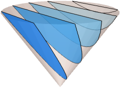
region = [image];Minimize the radius ![]() subject to the constraints
subject to the constraints ![]() :
:
constraints = Table[Norm[Inactive[Plus][pi, -c]] ≤ r, {pi, MeshCoordinates[region]}];res = SecondOrderConeOptimization[r, constraints, {r, c∈Vectors[3]}]Show[Graphics3D[{Opacity[0.2], Red, Ball[c, r] /. res}], region]The minimal enclosing ball can be found efficiently using BoundingRegion:
BoundingRegion[region, "MinBall"]Facility Location Problems (3)
A company wants to open a new factory. The factory needs raw materials from five warehouses. The transportation cost per unit distance between the new factory and warehouses is:
costPerUnitDist = {1000, 1500, 2000, 1000, 1500};Let ![]() be the distance between factory and warehouses
be the distance between factory and warehouses ![]() The objective is to minimize
The objective is to minimize ![]() :
:
totalCost = costPerUnitDist.d;The five warehouses are located at:
pos = {{0, 0}, {1, 0}, {3 / 2, 1}, {-1 / 2, 1}, {1 / 2, 3 / 2}};The new factory must be located such that ![]() :
:
constraints = Table[Norm[Inactive[Plus][pos[[i]], -p]] ≤ Indexed[d, i], {i, Length[pos]}];Find the optimal distances between the new factory and the warehouses:
res = SecondOrderConeOptimization[totalCost, constraints, {d, p∈Vectors[2]}]The new factory location is closer to the warehouses where the transportation costs are higher:
ListPlot[Thread[{pos}], Sequence[...], Epilog -> {Red, PointSize[0.03], Point[p /. res]}]A company wants to open a two new factories. The factories need raw materials from five warehouses. The transportation cost per unit distance between the new factories and warehouses is:
costPerUnitDist = (| | | | | |
| ---- | ---- | ---- | ---- | ---- |
| 1000 | 1500 | 2000 | 1000 | 1500 |
| 1500 | 1500 | 1000 | 2000 | 1500 |);
nFactories = 2;
nWarehouses = 5;Let ![]() be the distance between factory
be the distance between factory ![]() and warehouse
and warehouse ![]() The objective is to minimize
The objective is to minimize ![]() :
:
totalCost = Flatten[costPerUnitDist].d;The five warehouses are located at:
pos = {{0, 0}, {1, 0}, {3 / 2, 1}, {-1 / 2, 1}, {1 / 2, 3 / 2}};The new factories must be located such that ![]() :
:
constraints = Table[Norm[Inactive[Plus][pos[[i]], -q[j]]] ≤ Indexed[d, i + nWarehouses * (j - 1)], {i, nWarehouses}, {j, nFactories}];Find the optimal distances between the new factory and the warehouses:
res = SecondOrderConeOptimization[totalCost, constraints, {d∈Vectors[nFactories * nWarehouses], q[1]∈Vectors[2], q[2]∈Vectors[2]}]The new factory location is closer to the warehouses where the transportation costs are higher:
Show[ListPlot[Thread[{pos}], Sequence[...]], ListPlot[{{q[1]}, {q[2]}} /. res, IconizedObject[«Rule»]]]Find the minimum number and location of warehouses to construct that can supply the company's five retail stores. There are five potential sites. The cost of transporting one unit of product from a given warehouse to a given store is given by a table:
transportCosts = {{4, 5, 6, 8, 10}, {6, 4, 3, 5, 8},
	{9, 7, 4, 3, 4}, {5, 6, 4, 8, 9}, {7, 8, 6, 10, 8}};TableForm[transportCosts, Rule[...]]
The positions of the retail stores ![]() are:
are:
retailStorePos = {{0, 0}, {1, 0}, {3 / 2, 1}, {-1 / 2, 1}, {1 / 2, 3 / 2}};The demand in the retail stores is:
retailStoreDemand = {80, 270, 250, 160, 180};For every warehouse, there is a $1000 overhead cost:
overheadCost = {1000, 1000, 1000, 1000, 1000};Each warehouse can hold a maximum of 500 units of product:
warehouseCapacity = {500, 500, 500, 500, 500};Let ![]() be the number of units that is transported from warehouse
be the number of units that is transported from warehouse ![]() to store
to store ![]() . The demand constraint is:
. The demand constraint is:
demandConstraint = Total[x, {2}] == retailStoreDemand;Let ![]() be a binary decision vector such that if
be a binary decision vector such that if ![]() , then warehouse
, then warehouse ![]() is constructed. The supply constraint is:
is constructed. The supply constraint is:
supplyConstraint = Total[x]Inactive[Times][warehouseCapacity, y];The new warehouses must be located such that ![]() :
:
positionConstraint = Table[Inactive[Norm][Inactive[Plus][
	Indexed[y, j] * retailStorePos[[i]], -q[j]]] ≤ Indexed[d, {i, j}], {i, 5}, {j, 5}];
The objective is to minimize the number of warehouses, the transportation cost of goods and the distance of the warehouse from the retail store:
objective = Inactive[Plus][overheadCost.y, Total[transportCosts.x, 2], Total[Inactive[Times][transportCosts, d], 2]];vars = Flatten[{x∈Matrices[{5, 5}, Integers], y∈Vectors[5, Integers], d∈Matrices[{5, 5}], Table[q[i]∈Vectors[2], {i, 5}]}];Solve the minimum number and positions of the warehouses:
res = SecondOrderConeOptimization[objective, {demandConstraint,
supplyConstraint, positionConstraint, 0y1, x0, d0}, vars];The number of units to be transported from warehouse ![]() to store
to store ![]() is:
is:
TableForm[(x /. res) /. 0 -> _, Rule[...]]The positions of the warehouses are:
warehousePos = Pick[Table[q[i], {i, 5}] /. res, y /. res, 1];
Graphics[{{Red, PointSize[0.02], Point[retailStorePos]}, {Blue, PointSize[0.02], Point[warehousePos]}}]
Data-Fitting Problems (6)
Find a linear fit to discrete data by minimizing ![]() subject to the constraints
subject to the constraints ![]() :
:
{a1, b1} = IconizedObject[«Block»];Using auxiliary variable ![]() , minimize
, minimize ![]() subject to
subject to ![]() :
:
SecondOrderConeOptimization[t, {a == a1, b == b1, Norm[a.x - b] ≤ t, x1}, {x, t}]Fit a fifth-order polynomial to discrete data by minimizing ![]() :
:
data = IconizedObject[«Block»];
dataplot = ListPlot[data, PlotRange -> All]
Construct the input data matrix using DesignMatrix:
a = DesignMatrix[data, Array[s^#&, 5], s];
b = data[[All, 2]];
Find the coefficients of the quadratic curve by minimizing ![]() subject to
subject to ![]() :
:
res = SecondOrderConeOptimization[t, Norm[Inactive[Plus][a.c, -b]] ≤ t, {c, t}]Show[dataplot, Plot[Evaluate[(c /. res).Map[s^#&, Range[0, 5]]], {s, 0, 1}]]Find an approximating function to noisy data using bases ![]() such that the first and last points lie on the curve:
such that the first and last points lie on the curve:
data = IconizedObject[«Block»];
dataplot = ListPlot[data, PlotStyle -> Red, PlotRange -> All]
The approximating function will be ![]() :
:
bases = Sqrt[1 + (x - #) ^ 2]& /@ Subdivide[-3, 3, 10];
a = DesignMatrix[data, bases, x, IncludeConstantBasis -> False];
b = data[[All, 2]];
Find the coefficients of the approximating function by minimizing ![]() subject to
subject to ![]() :
:
res = SecondOrderConeOptimization[t, {Norm[Inactive[Plus][a.λ, -b]] ≤ t}, {λ, t}]Show[dataplot, Plot[Evaluate[bases.(λ /. res)], {x, -3, 3}]]Find a robust linear fit to discrete data by minimizing ![]() , where
, where ![]() is a known regularization parameter:
is a known regularization parameter:
{a, b} = IconizedObject[«Block»];
dataplot = ListPlot[b, PlotRange -> All]
Fit the line by minimizing ![]() subject to
subject to ![]() :
:
With[{λ = 1},
	res = SecondOrderConeOptimization[t + λ Total[s], {Norm[Inactive[Plus][a.x, -b]] ≤ t, VectorLessEqual[{Abs[x] - s, 0}]}, {t, x, s∈Vectors[2]}]]
A plot of the line shows that it is robust to the outliers:
Show[dataplot, Plot[Evaluate[x.{1, y} /. res], {y, 1, 30}]]The robust ![]() fitting can also be obtained using the function Fit:
fitting can also be obtained using the function Fit:
Fit[{a, b}, NormFunction -> Norm, FitRegularization -> {"L1", 1}]Excess regularization will lead to the fit becoming increasingly insensitive to data:
rvals = {0, 10, 50, 75, 90};
lines = Table[
	res = SecondOrderConeOptimization[t + λ Total[s], {Norm[Inactive[Plus][a.x, -b]] ≤ t, VectorLessEqual[{Abs[x] - s, 0}]}, {t, x, s∈Vectors[2]}];
x.{1, y} /. res, {λ, rvals}];Show[dataplot, Plot[Evaluate[lines], {y, 1, 30}, PlotStyle -> {Red, Green, Blue, Brown, Magenta}, PlotLegends -> N[rvals]]]Cardinality constrained least squares: minimize ![]() such that
such that ![]() has at most
has at most ![]() nonzero elements:
nonzero elements:
m  = 33; n = 7;k = 4;
SeedRandom[1234];
a = RandomReal[{-1, 1}, {m, n}];
b = RandomReal[{-1, 1}, m];
Let ![]() be a decision vector such that if
be a decision vector such that if ![]() , then
, then ![]() is nonzero. The decision constraints are:
is nonzero. The decision constraints are:
decisionConstraints = {Total[z] ≤ k, 0z1, z∈Vectors[n, Integers]};To model constraint ![]() when
when ![]() , chose a large constant
, chose a large constant ![]() such that
such that ![]() :
:
coeffConstraint = -100 zx100z;Using epigraph transformation, the objective is to minimize ![]() subject to
subject to ![]() :
:
epigraphConstraint = Norm[Inactive[Plus][a.x, -b]] ≤ t;Solve the cardinality constrained least-squares problem:
SecondOrderConeOptimization[t, {epigraphConstraint,
	decisionConstraints, coeffConstraint}, {t, x, z}]
The subset selection can also be done more efficiently with Fit using ![]() regularization. First, find the range of regularization parameters that uses at most
regularization. First, find the range of regularization parameters that uses at most ![]() basis functions:
basis functions:
nterms = Table[{λ, Length[Fit[{a, b}, FitRegularization -> {"L1", λ}]
	["NonzeroPositions"]]}, {λ, 1, 3, 0.02}];
λk = Mean[MinMax[Cases[nterms, {x_, k} -> x]]]
Find the nonzero terms in the ![]() regularized fit:
regularized fit:
fitTerms = Flatten[Fit[{a, b}, FitRegularization -> {"L1", λk}]
	["NonzeroPositions"]]
Find the fit with just these basis terms:
Fit[{a[[All, fitTerms]], b}]Find the best subset of functions from a candidate set of functions to approximate given data:
refFun[x_] := Exp[-(5 * (x - 1 / 2)) ^ 2];
data = Table[{x, refFun[x]}, {x, 0, 1, 0.02}];
The approximating function will be ![]() :
:
basis = Join[Cos[Range[10] * Pi * x], Sin[Range[10] * Pi * x]];
qf = DesignMatrix[data, basis, x, IncludeConstantBasis -> False];
cf = data[[All, 2]];
A maximum of 5 basis functions are to be used in the final approximation:
functionConstraint = {Total[z] ≤ 5, 0z1};The coefficients associated with functions that are not chosen must be zero:
coeffConstraint = {-10 * zxz * 10};Using epigraph transformation, the objective is to minimize ![]() such that
such that ![]() :
:
epigraphConstraint = Norm[Inactive[Plus][qf.x, -cf]] ≤ t;Find the best subset of functions:
res = SecondOrderConeOptimization[t, {epigraphConstraint,
	functionConstraint, coeffConstraint}, {t, x,
	z∈Vectors[Last[Dimensions[qf]], Integers]}]
Compare the resulting approximation with the given data:
{coeffs, chosen} = {x, z} /. res;
fun = Total[Pick[basis * coeffs, chosen, 1]];
Plot[fun, {x, 0, 1}, Epilog -> Point[data], PlotRange -> All]
Classification Problems (2)
Find a quartic polynomial ![]() that robustly separates two sets of points in the plane:
that robustly separates two sets of points in the plane:
{set1, set2} = IconizedObject[«Block»];
dataplot = ListPlot[{set1, set2}, Sequence[...]]
The polynomial is defined as ![]() , with
, with ![]() :
:
d = 4;
poly[{x_, y_}] = Sum[Subscript[a, i, j]x^iy^j, {j, 0, d}, {i, 0, d - j}]
For separation, set 1 must satisfy ![]() and set 2 must satisfy
and set 2 must satisfy ![]() :
:
constraints = {Thread[Map[poly, set1] ≤ -1], Thread[Map[poly, set2] ≥ 1]};The objective is to minimize ![]() , which gives twice the thickness between
, which gives twice the thickness between ![]() and
and ![]() . Using the auxiliary variable
. Using the auxiliary variable ![]() , the objective function is transformed to the constraint
, the objective function is transformed to the constraint ![]() :
:
coeffs = Flatten[Table[Subscript[a, i, j], {j, 0, d}, {i, 0, d - j}]];
coeffConstraint = Norm[coeffs] ≤ t;
Find the coefficients ![]() by minimizing
by minimizing ![]() :
:
res = SecondOrderConeOptimization[t, {constraints, coeffConstraint}, Append[coeffs, t]]Visualize the separation of the sets using the polynomial:
Show[RegionPlot[Evaluate[poly[{x, y}] ≤ 0 /. res], {x, -2, 2}, {y, -2, 2}], dataplot, ImageSize -> 300]The value ![]() is the width in terms of level values of
is the width in terms of level values of ![]() , where there are no points:
, where there are no points:
quarticPoly1 = (poly[{x, y}] ≤ -1) /. res;
quarticPoly2 = (poly[{x, y}] ≤ 1) /. res;Show[RegionPlot[{quarticPoly1, quarticPoly2}, {x, -2, 2}, {y, -2, 2}, ImageSize -> 300], dataplot]Find a quartic polynomial ![]() that robustly separates two sets of points in 3D:
that robustly separates two sets of points in 3D:
{set1, set2} = IconizedObject[«Block»];
dataplot = ListPointPlot3D[{set1, set2}, IconizedObject[«Rule»]]
The polynomial is defined as ![]() , with
, with ![]() :
:
d = 4;
poly[{x_, y_, z_}] := Sum[Subscript[a, i, j, k] x^i y^j z^k, {i, 0, d}, {j, 0, d - i}, {k, 0, d - i - j}];
For separation, set 1 must satisfy ![]() and set 2 must satisfy
and set 2 must satisfy ![]() :
:
constraints = {Thread[Map[poly, set1] ≤ -1], Thread[Map[poly, set2] ≥ 1]};The objective is to minimize ![]() . Using transformation
. Using transformation ![]() , the objective is now to minimize
, the objective is now to minimize ![]() :
:
coeffs = Flatten[Table[Subscript[a, i, j, k], {i, 0, d}, {j, 0, d - i}, {k, 0, d - i - j}]];
coeffConstraint = Norm[coeffs] ≤ t;
Find the coefficients ![]() by minimizing
by minimizing ![]() :
:
res = SecondOrderConeOptimization[t, {constraints, coeffConstraint}, Append[coeffs, t]]Visualize the separation of the sets using the polynomial:
Show[RegionPlot3D[Evaluate[poly[{x, y, z}] ≤ 0 /. res], {x, -1.5, 1.5}, {y, -3, 1 / 2}, {z, -2, 2}, PlotStyle -> Directive[Yellow, Opacity[0.5]], Mesh -> None], dataplot]Structural Optimization Problems (1)
Find the shape of a hanging chain formed by ![]() spring links under a vertical load at the end of each link. The objective is to find the link positions
spring links under a vertical load at the end of each link. The objective is to find the link positions ![]() :
:
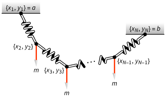
The potential energy due to gravity is ![]() , where
, where ![]() is the vertical load at each end and
is the vertical load at each end and ![]() is gravity:
is gravity:
n = 20;
gravityPE = m g Total[y];
The potential energy due to the tension in the spring link due to stretching is ![]() , where
, where ![]() is the stretch in spring link
is the stretch in spring link ![]() and
and ![]() is the stiffness of the spring. Using
is the stiffness of the spring. Using ![]() , the energy is transformed to
, the energy is transformed to ![]() :
:
springPE = k u;An additional constraint ![]() must be added due to the transformation:
must be added due to the transformation:
auxConstraint = Norm[t]^2 ≤ 2u;
energyConstraint = VectorGreaterEqual[{t, 0}];
The ends of the linked chain are clamped at positions (0,0) and (2,-1):
endConditions = {Indexed[x, 1] == 0, Indexed[y, 1] == 0, Indexed[x, n + 1] == 2, Indexed[y, n + 1] == -1};Each link has to satisfy the condition ![]() , where
, where ![]() is the resting length of each spring:
is the resting length of each spring:
linkConditions = Table[Inactive[Norm][{Indexed[x, i] - Indexed[x, i + 1], Indexed[y, i] - Indexed[y, i + 1]}] - Subscript[l, 0] ≤ Indexed[t, i], {i, 1, n}];params = {k -> 500, m -> 1, g -> 9.81, Subscript[l, 0] -> 0.25};The final objective function is the sum of gravity and spring potential energy that must be minimized:
totalEnergy = (gravityPE + springPE) /. params;Find the end points of each of the spring links:
res = SecondOrderConeOptimization[totalEnergy, {auxConstraint, endConditions, linkConditions} /. params, {t∈Vectors[n], x∈Vectors[n + 1], y∈Vectors[n + 1], u}];Visualize the shape of the resulting spring chain:
ListLinePlot[Transpose[{x, y} /. res], PlotMarkers -> Automatic]The stretch is greatest for the links near the ends of the link chain. Links 11 and 12 have the least elongation:
BarChart[Evaluate[t /. res], ChartLabels -> Range[n], ImageSize -> 300]Portfolio Optimization (1)
Find the distribution of capital to invest in six stocks to maximize return while minimizing risk:
{μ, Σ} = Block[...];Let ![]() be the percentage of total investment made in stock
be the percentage of total investment made in stock ![]() . The return is given by
. The return is given by ![]() where
where ![]() is a vector of expected return value of each individual stock:
is a vector of expected return value of each individual stock:
return = μ.w;The risk is given by ![]() ,
, ![]() is a risk-aversion parameter and
is a risk-aversion parameter and ![]() :
:
risk = w.Σ.w;
riskConstraint = risk ≤ s;
The objective is to maximize return while minimizing risk for a specified risk-aversion parameter:
objective[α_ ? NumericQ] := -(return - α s);The percentage of investment ![]() must be greater than 0 and must add to 1:
must be greater than 0 and must add to 1:
weightConstraints = {w0, Total[w] == 1};Compute the returns and corresponding risk for a range of risk-aversion parameters:
frontier = Table[res = Quiet@SecondOrderConeOptimization[
	objective[α], {riskConstraint, weightConstraints}, {w, s}];
	{risk, return} /. res, {α, Subdivide[0.0001, 3, 100]}];
The optimal ![]() over a range of
over a range of ![]() gives an upper-bound envelope on the tradeoff between return and risk:
gives an upper-bound envelope on the tradeoff between return and risk:
randomRiskReturns = Table[{risk, return}, {w, Map[...]}];
Show[ListPlot[frontier, ...], ListPlot[randomRiskReturns, Rule[...]]]
Compute the percentage of investment ![]() for a specified number of risk-aversion parameters:
for a specified number of risk-aversion parameters:
riskAversionParameter = N@{1 / 100, 1 / 2, 1, 10, 100, 1000};
res = Table[{α, return, w} /.
	Quiet@SecondOrderConeOptimization[objective[α], {riskConstraint, weightConstraints}, {w, s}], {α, riskAversionParameter}];
Increasing the risk-aversion parameter ![]() causes the investment to be diversified:
causes the investment to be diversified:
Legended[BarChart[res[[All, -1]], ...], SwatchLegend[...]]Increasing the risk-aversion parameter ![]() causes the return on investment to decrease:
causes the return on investment to decrease:
ListLogLogPlot[res[[All, 1 ;; 2]], ...]Non-negative Matrix Factorization (1)
Given ![]() , find matrices
, find matrices ![]() and
and ![]() such that
such that ![]() :
:
SeedRandom[123];
r = 4;
A = RandomReal[5, {10, r}].RandomReal[5, {r, 20}];
The objective is to minimize ![]() . This is done by fixing
. This is done by fixing ![]() and
and ![]() alternatively and iteratively solving until convergence. Specify the constraints:
alternatively and iteratively solving until convergence. Specify the constraints:
{n, m} = Dimensions[A];
WCons = Table[Norm[-A[[i]] + W[i].h] ≤ Indexed[t, i], {i, n}];
HCons = Table[Norm[-A[[All, j]] + w.H[j]] ≤ Indexed[s, j], {j, m}];WVars = Table[W[i]∈Vectors[r, NonNegativeReals], {i, n}];
HVars = Table[H[j]∈Vectors[r, NonNegativeReals], {j, m}];Specify an initial guess for ![]() and
and ![]() :
:
W1 = RandomReal[5, {n, r}];
H1 = RandomReal[5, {r, m}];count = 0;
err = Quiet@Reap[While[Sow[Norm[A - W1.H1]] ≥ 10^-3 && (count++) ≤ 100,
res = SecondOrderConeOptimization[Total[t], {h == H1, WCons}, Join[WVars, {t∈Vectors[n]}], Method -> "CSDP"];
W1 = WVars[[All, 1]] /. res;
res = SecondOrderConeOptimization[Total[s], {w == W1, HCons}, Join[HVars, {s∈Vectors[m]}], Method -> "CSDP"];
H1 = Transpose[HVars[[All, 1]] /. res];
]];ListLogPlot[err[[2, 1]], PlotRange -> All]Investment Problems (3)
Find the number of stocks to buy from four stocks such that a minimum $1000 dividend is received and risk is minimized. The expected return value and the covariance matrix ![]() associated with the stocks are:
associated with the stocks are:
{returnValue, R} = Block[...];The unit price for the four stocks is $1. Each stock can be allocated a maximum of $2500:
capitalConstraint = x2500;The investment must yield a minimum of $1000:
returnConstraint = returnValue.x1000;A negative stock cannot be bought:
minStock = x0;Using epigraph transformation, the risk, given by ![]() , is converted into a constraint:
, is converted into a constraint:
riskConstraint = x.R.x ≤ t;The total amount to spend on each stock is found by minimizing the risk given by:
res = SecondOrderConeOptimization[t, {riskConstraint, capitalConstraint,
	returnConstraint, minStock}, {t, x∈Vectors[4, Integers]}]
The total investment to get a minimum of $1000 is:
Total[x /. res]Find the number of stocks to buy from four stocks with an option to short-sell such that a minimum dividend of $1000 is received and the overall risk is minimized:
{returnValue, R} = IconizedObject[«Block»];The capital constraint, return on investment constraints and risk constraint are:
constraints = {x2500, returnValue.x1000, x.R.x ≤ t};A short-sale option allows the stock to be sold. The optimal number of stocks to buy/short-sell is found by minimizing the risk given by the objective ![]() :
:
res = SecondOrderConeOptimization[t, constraints, {t, x∈Vectors[4, Integers]}]The second stock can be short-sold. The total investment to get a minimum of $1000 due to the short-selling is:
Total[x /. res]Without short-selling, the initial investment will be significantly more:
Total[x /. SecondOrderConeOptimization[t, {constraints, x0}, {t, x∈Vectors[4, Integers]}]]Find the best combination of six stocks to invest in out of a possible 20 candidate stocks, so as to maximize return while minimizing risk:
{μ, Σ} = Block[...];Let ![]() be the percentage of total investment made in stock
be the percentage of total investment made in stock ![]() . The return is given by
. The return is given by ![]() , where
, where ![]() is a vector of the expected return value of each individual stock:
is a vector of the expected return value of each individual stock:
return = μ.w;The risk is given by ![]() ,
, ![]() is a risk-aversion parameter and
is a risk-aversion parameter and ![]() :
:
risk = w.Σ.w;
riskConstraint = risk ≤ s;
The objective is to maximize return while minimizing risk for a specified risk-aversion parameter:
objective = s - return;Let ![]() be a decision vector such that if
be a decision vector such that if ![]() , then that stock is bought. Six stocks have to be chosen:
, then that stock is bought. Six stocks have to be chosen:
decisionConstraints = {Total[x] == 6, 0x1};The percentage of investment ![]() must be greater than 0 and must add to 1:
must be greater than 0 and must add to 1:
weightConstraints = {0wx, Total[w] == 1};Find the optimal combination of stocks that minimizes the risk while maximizing return:
res = SecondOrderConeOptimization[objective, {riskConstraint, decisionConstraints, weightConstraints}, {s, w, x∈Vectors[20, Integers]}];The optimal combination of stocks is:
stockPicks = Flatten[Position[x /. res, 1]]The percentages of investment to put into the respective stocks are:
(w /. res)[[stockPicks]]Trajectory Optimization Problems (1)
Find the shortest path between two points while avoiding obstacles. Specify the obstacle:
SeedRandom[12345];mesh = ConvexHullMesh[RandomReal[{.2, .8}, {10, 2}]];Extract the half-spaces that form the convex obstacle:
{a, b} = LinearOptimization[0, {}, Element[x, mesh], "LinearInequalityConstraints"];Specify the start and end points of the path:
start = {0, 0};
end = {1, 1};
The path can be discretized using ![]() points. Let
points. Let ![]() represent the position vector:
represent the position vector:
n = 15;
pvars = Table[Element[p[i], Vectors[2, Reals]], {i, 1, n}];
The objective is to minimize ![]() . Using epigraph transformation, the objective can be transformed to
. Using epigraph transformation, the objective can be transformed to ![]() subject to the constraints
subject to the constraints ![]() :
:
tvars = Table[t[i], {i, n - 1}];
transformationConstraint = Table[Norm[p[i + 1] - p[i]] ≤ t[i], {i, n - 1}];
objective = Total[tvars];
Specify the end point constraints:
endPointConstraints = {p[1] == start, p[n] == end};The distance between any two subsequent points should not be too large:
maxDist = 1.5Norm[start - end] / n;
separationConstraints = Table[-maxDist t[i]maxDist ,
{i, n - 1}];A point ![]() is outside the object if at least one element of
is outside the object if at least one element of ![]() is less than zero. To enforce this constraint, let
is less than zero. To enforce this constraint, let ![]() be a decision vector and
be a decision vector and ![]() be the
be the ![]()
![]() element of
element of ![]() such that
such that ![]() , then
, then ![]() and
and ![]() is large enough such that
is large enough such that ![]() :
:
m = 10;
zvars = Table[Element[z[i], Vectors[Length[a], Integers]], {i, n}];
binaryConstraints = Table[0 z[i] 1, {i, n}];
avoidanceConstraints = Table[{Inactive[Plus][a.p[i], b] m z[i], Total[z[i]] ≤ Length[a] - 1}, {i, n}];Find the minimum distance path around the obstacle:
res = SecondOrderConeOptimization[objective, {endPointConstraints, transformationConstraint, separationConstraints, binaryConstraints, avoidanceConstraints}, Join[pvars, tvars, zvars]];path = Table[p[i], {i, n}] /. res;
Show[mesh, Graphics[{Point[path], Line[path]}]]To avoid potential crossings at the edges, the region can be inflated and the problem solved again:
newMesh = RegionResize[mesh, {Scaled[1.3], Scaled[1.3]}];
{a, b}  =   LinearOptimization[0, {}, Element[x, newMesh], "LinearInequalityConstraints"];
Get the new constraints for avoiding the obstacles:
avoidanceConstraints = Table[{Inactive[Plus][a.p[i], b] m z[i],
Total[z[i]] ≤ Length[a] - 1}, {i, n}];res = SecondOrderConeOptimization[objective, {endPointConstraints, transformationConstraint, separationConstraints, binaryConstraints, avoidanceConstraints}, Join[pvars, tvars, zvars]];Extract and display the new path:
path = Table[p[i], {i, n}] /. res;
Show[ mesh, Graphics[{Point[path], Line[path]}]]
Properties & Relations (8)
SecondOrderConeOptimization gives the global minimum of the objective function:
Subscript[x, min] = SecondOrderConeOptimization[x + y, {Norm[{x, y}] ≤ 1,
	Norm[{x - 1 / 2, y}] ≤ 1}, {x, y}, "PrimalMinimizerRules"]
Visualize the objective function:
Show[Plot3D[x + y, ...], Graphics3D[{Blue, PointSize[0.05],
	Point[{x, y, x + y} /. Subscript[x, min]]}]]
Minimize gives global exact results for quadratic optimization problems:
Minimize[{x + y, {Norm[{x, y}] ≤ 1, Norm[{x - 1 / 2, y}] ≤ 1}}, {x, y}]NMinimize can be used to obtain approximate results using global methods:
NMinimize[{x + y, {Norm[{x, y}] ≤ 1, Norm[{x - 1 / 2, y}] ≤ 1}}, {x, y}]FindMinimum can be used to obtain approximate results using local methods:
FindMinimum[{x + y, {Norm[{x, y}] ≤ 1, Norm[{x - 1 / 2, y}] ≤ 1}}, {x, y}]LinearOptimization is a special case of SecondOrderConeOptimization:
SecondOrderConeOptimization[x + 2y, {3x + 4y ≥ 5, x ≥ 0, y ≥ 0}, {x, y}]LinearOptimization[x + 2y, {3x + 4y ≥ 5, x ≥ 0, y ≥ 0}, {x, y}]//NQuadraticOptimization is a special case of SecondOrderConeOptimization:
QuadraticOptimization[x^2 + y^2 - 2x - 6y, {x + 2y ≥ 4, x ≤ 3}, {x, y}, {"PrimalMinimizer", "PrimalMinimumValue"}]Use auxiliary variable ![]() and minimize
and minimize ![]() with the additional constraint
with the additional constraint ![]() :
:
SecondOrderConeOptimization[t, {x^2 + y^2 - 2x - 6y ≤ t, {x + 2y ≥ 4, x ≤ 3}}, {x, y, t}, {"PrimalMinimizer", "PrimalMinimumValue"}]SemidefiniteOptimization is a generalization of SecondOrderConeOptimization:
SecondOrderConeOptimization[x + y, {Norm[{x, y}] ≤ 1,
Norm[{x - 1 / 2, y}] ≤ 1}, {x, y}]SemidefiniteOptimization[x + y, {Norm[{x, y}] ≤ 1,
Norm[{x - 1 / 2, y}] ≤ 1}, {x, y}]ConicOptimization is a generalization of SecondOrderConeOptimization:
SecondOrderConeOptimization[x + y, {Norm[{x, y}] ≤ 1, Norm[{x - 1 / 2, y}] ≤ 1}, {x, y}]ConicOptimization[x + y, {Norm[{x, y}] ≤ 1, Norm[{x - 1 / 2, y}] ≤ 1}, {x, y}]Possible Issues (5)
Constraints specified using strict inequalities may not be satisfied for certain methods:
{obj, cons} = {t, {x ^ 2 + x + y ≤ t, x - 2y ≤ 3, x > 1, y > 0}};The reason is that SecondOrderConeOptimization solves ![]() :
:
cons /. SecondOrderConeOptimization[obj, cons, {x, y, t}]The minimum value of an empty set or infeasible problem is defined to be ![]() :
:
SecondOrderConeOptimization[t, {x ^ 2 ≤ t, x ≤ 0, x ≥ 1}, {x, t}, "PrimalMinimumValue"]The minimizer is Indeterminate:
SecondOrderConeOptimization[t, {x ^ 2 ≤ t, x ≤ 0, x ≥ 1}, {x, t}]The minimum value for an unbounded set or unbounded problem is ![]() :
:
SecondOrderConeOptimization[t, {x ^ 2 + y ≤ t, x ≤ 0 ≤ 1}, {x, y, t}, "PrimalMinimumValue"]The minimizer is Indeterminate:
SecondOrderConeOptimization[t, {x ^ 2 + y ≤ t, x ≤ 0 ≤ 1}, {x, y, t}]Dual related solution properties for mixed-integer problems may not be available:
SecondOrderConeOptimization[t, {2x^2 + 20y^2 + 6x y + 5x ≤ t, -x + y ≥ 2}, {x∈Integers, y, t}, {"DualMaximumValue", "DualMaximizer", "DualityGap"}]Constraints with complex values need to be specified using vector inequalities:
{q, c} = {{{2, 1 + I}, {1 - I, 1}}, {2, 3}};
SecondOrderConeOptimization[{1, 2}.x, (1 / 2) * x.q.x + c.x1, x∈Vectors[2, Reals]]Just using Less will not work even when both sides are real in theory:
{q, c} = {{{2, 1 + I}, {1 - I, 1}}, {2, 3}};
SecondOrderConeOptimization[{1, 2}.x, (1 / 2) * x.q.x + c.x < 1, x∈Vectors[2, Reals]]Text
Wolfram Research (2019), SecondOrderConeOptimization, Wolfram Language function, https://reference.wolfram.com/language/ref/SecondOrderConeOptimization.html (updated 2020).
CMS
Wolfram Language. 2019. "SecondOrderConeOptimization." Wolfram Language & System Documentation Center. Wolfram Research. Last Modified 2020. https://reference.wolfram.com/language/ref/SecondOrderConeOptimization.html.
APA
Wolfram Language. (2019). SecondOrderConeOptimization. Wolfram Language & System Documentation Center. Retrieved from https://reference.wolfram.com/language/ref/SecondOrderConeOptimization.html