

RayleighDistribution
表示尺度参数为 σ 的瑞利分布.
更多信息
- 当
 时,在瑞利分布中,
 的概率密度与
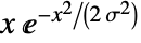 成正比,当
 时为0. »
- RayleighDistribution 允许 σ 是任意正实数.
- RayleighDistribution 允许 σ 为有任意单位量纲的量. »
- RayleighDistribution 可以与 Mean、CDF 和 RandomVariate 等函数一起使用. »
背景
- RayleighDistribution[σ] 表示在区间
 上支持的连续统计分布,参数是正实数 σ(称为“尺度参数”),确定了概率密度函数(PDF)的整体行为. 普遍来说,Rayleigh 分布的概率密度函数是具有一个峰(即全局最大值)的单峰函数,虽然它的整体形状(高度、扩展度和最大值的水平位置)由 σ 的值确定. 另外,概率密度函数的尾部是“瘦”的,因为对于较大的
 值,概率密度函数呈指数级下降,而不是呈几何级下降. (可以通过分析分布的 SurvivalFunction 使该行为定量精确.)
- Rayleigh 分布顾名思义是由 Lord Rayleigh 在1880年代初期作为求解声学中特定问题的工具. 在数学中,Rayleigh 分布是
 中从原点到点
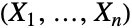 的距离的概率距离,其中变量
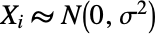 全是独立相同分布的正态变量. 进一步, Rayleigh 分布已经证明可以对各种现象建模,包括二维随机游走和电真空装置生产过程中的缺陷,并且是由泊松过程产生的空间配置中单独和最近邻之间距离的分布.
- RandomVariate 可用于给出一个或多个机器精度或任意精度(后者通过 WorkingPrecision 选项)的 Rayleigh 分布的伪随机变元. Distributed[x,RayleighDistribution[σ]],更简洁的表示为 xRayleighDistribution[σ],可用于论断随机变量 x 服从 Rayleigh 分布. 然后这类论断可用于诸如 Probability、NProbability、Expectation 和 NExpectation 等函数中.
- 概率密度和累积分布函数可以通过使用 PDF[RayleighDistribution[σ],x] 和 CDF[RayleighDistribution[σ],x] 给出. 均值、中位数、方差、原始矩和中心矩可以分别使用 Mean、Median、Variance、Moment 和 CentralMoment 计算.
- DistributionFitTest 可用于检验给定的数据集是否与 Rayleigh 分布相一致, EstimatedDistribution 可用于通过给定数据估计 Rayleigh 参数分布,而 FindDistributionParameters 可用于将数据拟合为 Rayleigh 分布. ProbabilityPlot 可用于生成已知数据相对于符号式 Rayleigh 分布的 CDF 图形,而 QuantilePlot 可用于生成已知数据相对于符号式 Rayleigh 分布的分位数的分位数图形.
- TransformedDistribution 可用于表示经过变换的 Rayleigh 分布,CensoredDistribution 可用于表示在上限和下限值之间删失值的分布,TruncatedDistribution 可用于表示在上限和下限值之间截断值的分布. CopulaDistribution 可用于构建包含 Rayleigh 分布的更高维分布,而 ProductDistribution 可用于计算独立分量分布涉及 Rayleigh 分布的联合分布.
- RayleighDistribution 和若干其它分布有关. RayleighDistribution 与 ChiDistribution 和ChiSquareDistribution 有关,因为 RayleighDistribution[1] 的概率密度函数和累积分布函数分别与 ChiDistribution[2] 的概率密度函数和 ChiSquareDistribution[2] 的累积分布函数完全相同. RayleighDistribution 可以作为 RiceDistribution、GammaDistribution 和 WeibullDistribution 的特例实现,因为 RayleighDistribution[σ] 的概率密度函数等价于 RiceDistribution[0,σ]、GammaDistribution[1,σ
 , 2, 0] 和 WeibullDistribution[2,σ
 ],而且作为 ExponentialDistribution 和 BeniniDistribution 的变换 (TransformedDistribution) . RayleighDistribution 也与 NormalDistribution, BinormalDistribution, LaplaceDistribution, SuzukiDistribution, LogNormalDistribution 和 KDistribution 相关.
范例
打开所有单元 关闭所有单元基本范例 (4)
Plot[Table[PDF[RayleighDistribution[σ], x], {σ, {.5, 1, 2}}]//Evaluate, {x, 0, 6}, Filling -> Axis, PlotRange -> All]PDF[RayleighDistribution[σ], x]Plot[Table[CDF[RayleighDistribution[σ], x], {σ, {.5, 1, 2}}]//Evaluate, {x, 0, 6}, Filling -> Axis, PlotRange -> All]CDF[RayleighDistribution[σ], x]Mean[RayleighDistribution[σ]]N[%]Variance[RayleighDistribution[σ]]N[%]Median[RayleighDistribution[σ]]N[%]范围 (7)
data = RandomVariate[RayleighDistribution[2], 10 ^ 4];Show[
Histogram[data, 20, "PDF"],
Plot[PDF[RayleighDistribution[2], x], {x, 0, 8}, PlotStyle -> Thick]]sample = RandomVariate[RayleighDistribution[3], 10 ^ 3];edist = EstimatedDistribution[sample, RayleighDistribution[σ]]Show[Histogram[sample, Automatic, "PDF"], Plot[PDF[edist, x], {x, 0, 10}, PlotStyle -> Thick]]Skewness[RayleighDistribution[σ]]N[%]Kurtosis[RayleighDistribution[σ]]N[%]FormulaGrid[list_, type_] := Grid[...]FormulaGrid[Table[Moment[RayleighDistribution[σ], k], {k, 5}], M]Moment[RayleighDistribution[σ], r]FormulaGrid[Table[CentralMoment[RayleighDistribution[σ], k]//Factor, {k, 5}], CM]FormulaGrid[Table[FactorialMoment[RayleighDistribution[σ], k]//Factor, {k, 5}], FM]FormulaGrid[Table[Cumulant[RayleighDistribution[σ], k]//Factor, {k, 5}], C]Plot[Table[HazardFunction[RayleighDistribution[σ], x], {σ, {0.5, 0.75, 1}}]//Evaluate, {x, 0, 4}, Filling -> Axis]HazardFunction[RayleighDistribution[σ], x]Plot[Table[Quantile[RayleighDistribution[σ], q], {σ, {0.5, 1, 2}}]//Evaluate, {q, 0, 1}, Filling -> Axis]Quantile[RayleighDistribution[σ], q]在参数中对 Quantity 使用的一致性产生了 QuantityDistribution:
serviceTime𝒟 = RayleighDistribution[Quantity[10, "Years"]]Mean[serviceTime𝒟]//N应用 (7)
Table[Arrow[{{0, 0}, RandomVariate[NormalDistribution[], 2]}], {100}]//Graphicsvectors = RandomVariate[NormalDistribution[], {10^4, 2}];Show[Histogram[Apply[ArcTan, vectors, {1}], Automatic, "PDF"], Plot[PDF[UniformDistribution[{-π, π}], x], {x, -π, π}, PlotStyle -> Thick]]Show[Histogram[Map[Norm, vectors], 25, "PDF"], Plot[PDF[RayleighDistribution[1], x], {x, 0, 5}, PlotStyle -> Thick]]TransformedDistribution[Norm[{u, v}], {uNormalDistribution[], vNormalDistribution[]}]某个产品失效的时间服从参数为 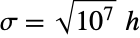 的瑞利分布. 求产品在 4000、4500 和 5000 小时处的可靠性. 可靠性也可称为生存概率:
time𝒟 = RayleighDistribution[Quantity[Sqrt[10^7], "Hours"]]Table[SurvivalFunction[time𝒟, t], {t, Quantity[{4000., 4500., 5000.}, "Hours"]}]SurvivalFunction[RayleighDistribution[σ], t]HazardFunction[RayleighDistribution[σ], t]rs = SurvivalFunction[RayleighDistribution[σ1], t]SurvivalFunction[RayleighDistribution[σ2], t]//PiecewiseExpandrp = 1 - (1 - SurvivalFunction[RayleighDistribution[σ1], t])(1 - SurvivalFunction[RayleighDistribution[σ2], t])//PiecewiseExpand

Block[{σ1 = 2, σ2 = 3}, Plot[{Legended[rs, "in series"], Legended[rp, "in parallel"]}, {t, 0, 10}]]一个向量具有两个分量,这两个分量都服从正态分布. 求该向量的长度的分布:
𝒟 = TransformedDistribution[Norm[{u, v}], {uNormalDistribution[], vNormalDistribution[]}]Plot[PDF[𝒟, x], {x, 0, 5}, Filling -> Axis]Mean[𝒟]ListPlot[{RandomVariate[𝒟, 30], {{0, Mean[𝒟]}, {30, Mean[𝒟]}}}, Joined -> {False, True}, Filling -> Axis, AxesOrigin -> {0, 0}]RayleighDistribution 可以用来近似风速:
wind = WeatherData["Copenhagen", "WindSpeed", {{2006, 1, 1}, {2009, 12, 31}, "Day"}]windEstimate = EstimatedDistribution[wind, RayleighDistribution[σ]]Show[Histogram[wind, Automatic, "PDF", AxesLabel -> Automatic], Plot[PDF[windEstimate, Quantity[x, "km/h"]], {x, 0, 35}, PlotStyle -> Thick]]Probability[x > Quantity[30, "Kilometers"/"Hours"], xwindEstimate]Mean[windEstimate]ListPlot[{RandomVariate[windEstimate, 30], {{0, Mean[windEstimate]}, {30, Mean[windEstimate]}}}, Joined -> {False, True}, Filling -> Axis, AxesOrigin -> {0, 0}, AxesLabel -> {"days", Automatic}]令  为给定地点的高度最高的三分之一波浪的高度的均值. 可以用 RayleighDistribution 对该地点的波浪高度建模:
𝒟 = RayleighDistribution[H / 2];SurvivalFunction[𝒟, x]
Probability[x > H, x𝒟]N[%]Mean[𝒟]N[%]
ListPlot[RandomVariate[𝒟 /. H -> Quantity[12, "m"], 100], Joined -> True, AxesLabel -> Automatic]在衰减信道理论中,RayleighDistribution 用于在不存在直射信号的情况下,对衰减信号幅度建模. 求瞬时信噪比的分布,其中 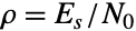 ,
 为符号的平均能量,
 为白噪声的谱密度:
SNRdist = TransformedDistribution[ρ u ^ 2, uRayleighDistribution[σ]];证明  为一个 ExponentialDistribution:
PDF[SNRdist, x]//Refine[#, ρ > 0]&PDF[ExponentialDistribution[1 / (2 ρ σ ^ 2)], x]FullSimplify[% - %%, x > 0]MomentGeneratingFunction[SNRdist, t]Mean[SNRdist](1 - Mean[SNRdist] t) ^ -1 == MomentGeneratingFunction[SNRdist, t]//FullSimplifyAF[dist_] := Variance[dist] / (Mean[dist]) ^ 2AF[SNRdist]属性和关系 (14)
当使用一个正因子为比例进行缩放时,所得的分布仍然是瑞利分布:
TransformedDistribution[k * u, uRayleighDistribution[σ]]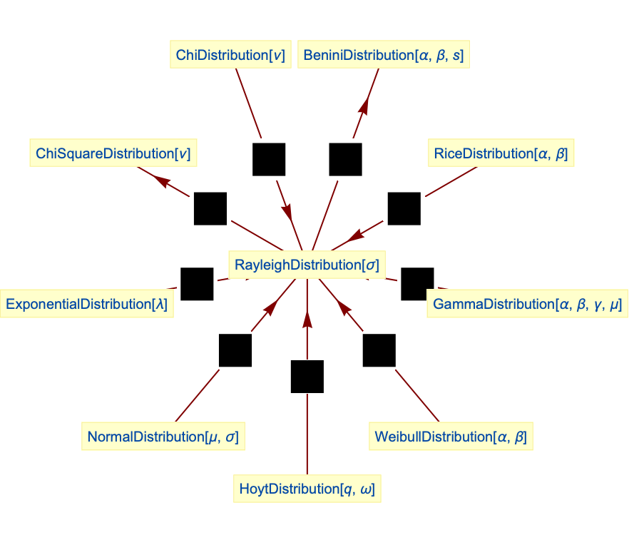
 的 RayleighDistribution 是 ChiDistribution 的一个特殊情况:
PDF[RayleighDistribution[1], x]PDF[ChiDistribution[2], x]Simplify[% - %%]当  时, RayleighDistribution 的平方是 ChiSquareDistribution 的一个特例:
CDF[RayleighDistribution[1], Sqrt[x]]CDF[ChiSquareDistribution[2], x]Simplify[% - %%, x > 0]瑞利分布是 RiceDistribution 的一个特例:
PDF[RayleighDistribution[β], x]PDF[RiceDistribution[0, β], x]% - %%RayleighDistribution 是 GammaDistribution 的一个特例:
PDF[GammaDistribution[1, σSqrt[2], 2, 0], x]PDF[RayleighDistribution[σ], x]% - %%BeniniDistribution 是瑞利分布的一个变换:
𝒟 = TransformedDistribution[Exp[u], uRayleighDistribution[σ]];PDF[𝒟, x]PDF[BeniniDistribution[0, 1 / (2σ ^ 2), 1], x]FullSimplify[% - %%, x > 1]TransformedDistribution[Norm[{u, v}], {uNormalDistribution[], vNormalDistribution[]}]NormalDistribution 和瑞利分布的参数混合是 LaplaceDistribution:
𝒟 = ParameterMixtureDistribution[NormalDistribution[μ, σ], σRayleighDistribution[ν]]瑞利分布与 BinormalDistribution 相关:
𝒟 = TransformedDistribution[Norm[{u, v}], {u, v}BinormalDistribution[{0, 0}, {σ, σ}, 0]];Block[{σ = 2}, Show[Histogram[RandomVariate[𝒟, 10 ^ 4], 20, "PDF"], Plot[PDF[RayleighDistribution[σ], x], {x, 0, 8}, PlotStyle -> Thick]]]瑞利分布是 WeibullDistribution 的一个特例:
PDF[WeibullDistribution[2, Sqrt[2]σ], x]PDF[RayleighDistribution[σ], x]% - %%瑞利分布可以通过 ExponentialDistribution 的变换获得:
TransformedDistribution[Sqrt[2 u], uExponentialDistribution[1 / σ ^ 2], Assumptions -> σ > 0]PDF[RayleighDistribution[σ], x] === PDF[%, x]SuzukiDistribution 可以从 LogNormalDistribution 和瑞利分布得到:
𝒟 = TransformedDistribution[u z, {uRayleighDistribution[1], zLogNormalDistribution[μ, ν]}];Block[{μ = -1, ν = 1 / 5}, Show[Histogram[RandomVariate[𝒟, 10 ^ 4], 25, "PDF"], Plot[PDF[SuzukiDistribution[μ, ν], x], {x, 0, 2}, PlotStyle -> Thick]]]KDistribution 可以表示为 RayleighDistribution 和 GammaDistribution 的参数混合:
𝒟 = ParameterMixtureDistribution[RayleighDistribution[Sqrt[σ]], σGammaDistribution[α, β / (2α)]]可能存在的问题 (2)
当 σ 不是正实数时,RayleighDistribution 没有定义:
Mean[RayleighDistribution[-1]]
Mean[RayleighDistribution[σ]] /. {σ -> 3 + I}巧妙范例 (2)
Table[Arrow[{{0, 0}, RandomVariate[NormalDistribution[], 2]}], {100}]//Graphics所得的单变量分布在径向服从 RayleighDistribution:
RevolutionPlot3D[(1/2π)PDF[RayleighDistribution[1], r], {r, 0, 4}, PlotStyle -> Opacity[0.8], PlotPoints -> 35, Mesh -> None]Integrate[(1/2π)PDF[RayleighDistribution[1], r], {r, 0, ∞}, {θ, 0, 2π}]RevolutionPlot3D[CDF[RayleighDistribution[1], r], {r, 0, 4}, PlotStyle -> Opacity[0.8], PlotPoints -> 35, Mesh -> None]dist = RayleighDistribution[σ];cdf = Function[{x, σ}, Evaluate[CDF[dist, x]]];
ql = {0.025, 0.10, 0.25, 0.5, 0.75, 0.90, 0.975};
cl = Table[ColorData["Rainbow"][q], {q, Join[{0.0}, ql]}];Legended[Plot3D[PDF[dist, x], {x, 0, 1}, {σ, 0.1, 1}, PlotTheme -> "Marketing", MeshFunctions -> {cdf}, Mesh -> {ql}, MeshStyle -> GrayLevel[0.8], MeshShading -> cl, AxesLabel -> Automatic, BaseStyle -> Opacity[0.9], ImageSize -> 400, PlotPoints -> 50, PlotRange -> All], BarLegend["Rainbow", ql, LegendLabel -> "prob"]]文本
Wolfram Research (2007),RayleighDistribution,Wolfram 语言函数,https://reference.wolfram.com/language/ref/RayleighDistribution.html (更新于 2016 年).
CMS
Wolfram 语言. 2007. "RayleighDistribution." Wolfram 语言与系统参考资料中心. Wolfram Research. 最新版本 2016. https://reference.wolfram.com/language/ref/RayleighDistribution.html.
APA
Wolfram 语言. (2007). RayleighDistribution. Wolfram 语言与系统参考资料中心. 追溯自 https://reference.wolfram.com/language/ref/RayleighDistribution.html 年