


WhenEvent
更多信息和选项
- 在 NDSolve[eqns,…] 中,WhenEvent 表达式被包含在 eqns 中,被考虑为解的部分规范,尤其是分段或混合系统.
- WhenEvent 表达式可以用于 NDSolve、NDSolveValue、ParametricNDSolve、ParametricNDSolveValue、DSolve 和 DSolveValue.
- 对应于在 NDSolve 中 eqns 积分时,在特定时间
 的事件.
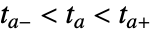
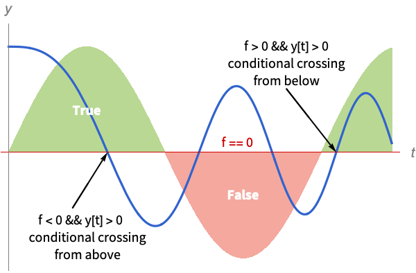
的事件. - 如果事件表达式以解的函数 f 显式给出,例如,在 f 的根处,事件变成 True,那么 WhenEvent 使用查找数值根的过程确定区间
 ,其中,
,其中, 是函数有根的时间. 显式给出事件的范例:
 -
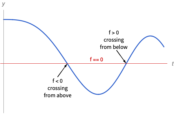
f0 解的变量函数 f 跨过零 f>0 从下面 f 跨过零 f<0 从上面 f 跨过零 Mod[t,  ]0
]0以固定间隔  ,时间变量
,时间变量  采样
采样 - 如果显式表达式为 ev,事件可以使用形式 ev && pred 以谓词 pred 为条件. 在这种情况下,事件只有在如果 pred 在事件函数的根处为 True 才会被触发.
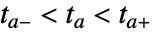
- 当事件以无法直接转换为上面的显式格式的形式给出,那么事件表达式被考虑为应该是 True 或 False 的谓词 pred. 在这种情况下,使用二等分找到区间
 .
. - 带有条件和事件作为谓词的显式事件的诠释略有不同. 如果可能最好使用显式事件,因为它们更有可能被检测到,并能更高效地找到根. »
- WhenEvent[{event1,…},action] 被处理为 {WhenEvent[event1,action],…}.
- 当 WhenEvent[event,{action1,action2,…}] 时,按序计算 action.
- 计算 action 得到的值被 WhenEvent 忽略,除非它有特殊的值被用于影响 NDSolve. 以下特殊值是被确认的:
-
"StopIntegration" 在  停止积分,返回解
"RestartIntegration" 在  重新开始积分
"CrossDiscontinuity" 积分到  ,推算并在
,推算并在  重新开始
重新开始"CrossSlidingDiscontinuity" 积分到  ,推算并检查滑动模式条件,在
  重新开始
重新开始"RemoveEvent" 去除事件 y[t]->val 把状态变量 y 改为 val d[t]->"DiscontinuitySignature" 改变不连续签名变量 d - 当 WhenEvent[f==0,d->"DiscontinuitySignature"] 时,不连续性是曲面 f==0,d 必须是一个接受值 {-1, 0, 1} 或 {-1, 1} 的离散变量,对于
 事件后,有效的设为 Sign[f].
 - WhenEvent 具有属性 HoldAll,因此,默认情况下,event 和 action 只有当变量被赋近似值时才被计算.
- WhenEvent 接受以下选项:
-
"DetectionMethod" Automatic 用于检测事件的方法 "LocationMethod" Automatic 用于在时间步骤中定位事件的方法 "IntegrateEvent" Automatic 是否积分事件函数 "Priority" Automatic 作用于同时发生事件的优先级 - "DetectionMethod" 可能的设置为:
-
Automatic 自动决定检测方法 "Sign" 使用一个符号变换 "DerivativeSign" 使用符号变换和时间导数 "Interpolation" 使用稠密解输出的插值 - "Sign" 检测方法具有最少的开销,但在快速变换的函数中可能错过事件. "Interpolation" 检测方法更强大,在每个步骤中可以检测多个事件.
- "LocationMethod" 可能的设置为:
-
Automatic 自动确定定位方法 "StepBegin" 在每个步骤开始前定位事件 "StepEnd" 在每个步骤结束时定位事件 "LinearInterpolation" 在步骤中线性插值 "Brent" 在一个步骤中使用 Brent 的根定位 - "IntegrateEvent" 可能的设置为:
-
Automatic 自动决定 False 不积分事件函数 True 积分事件函数 - "Priority" 的设置可以为任何整数或 Infinity. 在同时发生的事件中,将按排序的优先级顺序计算 action.
范例
打开所有单元 关闭所有单元基本范例 (1)
范围 (16)
事件 (6)
NDSolve[{x''[t] == -t x[t], x[0] == 0, x'[0] == 1, WhenEvent[x[t] == 1 / 2, Print[t]]}, x, {t, 0, 6}];


Plot[{x[t] /. %, 1 / 2}, {t, 0, 6}]NDSolve[{x''[t] == -t x[t], x[0] == 0, x'[0] == 1, WhenEvent[x[t] > 1 / 2, Print[t]]}, x, {t, 0, 6}];

NDSolve[{x''[t] == -t x[t], x[0] == 0, x'[0] == 1, WhenEvent[x[t] < 1 / 2, Print[t]]}, x, {t, 0, 6}];


Manipulate[{sol, samples} =
	Reap@NDSolve[{x'[t] == Sin[Exp[t]], x[0] == 0, WhenEvent[Mod[t, Δt] == 0, Sow[{t, x[t]}]]}, x, {t, 3}];
	Plot[x[t] /. sol, {t, 0, 3}, Epilog -> {PointSize[Medium], Red, Point@@samples}], {{Δt, 1}, .01, 2}, SaveDefinitions -> True]
以列表指定多个事件,当发生任一事件便触发行动(action):
NDSolve[{x''[t] + x[t] == 0, x'[0] == π, x[0] == 0, WhenEvent[{x[t] == 2, x[t] == -3}, x'[t] -> -x'[t]]}, x, {t, 0, 20}];Plot[{x[t] /. %, 2, -3}, {t, 0, 20}]


{sol, points} = Reap@NDSolve[{x'[t] == -y[t] - x[t] ^ 2, y'[t] == 2x[t] - y[t] ^ 3, x[0] == y[0] == 1, WhenEvent[y[t] == 0 && x[t] > 0, Sow[{x[t], y[t]}]]}, {x, y}, {t, 14}];ParametricPlot[Evaluate[{x[t], y[t]} /. sol], {t, 0, 14}, Epilog -> {PointSize[Medium], Red, Point@@points}, AxesLabel -> {x, y}]一般而言,事件可以是任何可以被检验为 True 的表达式:
Block[{eventtime = AbsoluteTime[] + 0.1},
	NDSolve[{x''[t]  + t x[t] == 0, x[0] == 1, x'[0] == 0, WhenEvent[AbsoluteTime[] > eventtime, eventtime += 0.3;Print[{AbsoluteTime[], t, x[t]}], "LocationMethod" -> "StepEnd"]}, x, {t, 0, 100}, WorkingPrecision -> 20]]
Button["Stop", stop = True]
stop = False;usol = NDSolveValue[{D[u[t, x], t, t] == D[u[t, x], x, x], u[0, x] == Exp[-10 x ^ 2], Derivative[1, 0][u][0, x] == 0, u[t, -10] == u[t, 10], WhenEvent[stop, "StopIntegration"]}, u, {t, 0, 100}, {x, -10, 10}, Method -> "StiffnessSwitching"]行为 (9)
NDSolve[{x''[t] == 0, x'[0] == 1, x[0] == 0, WhenEvent[{x[t] == 2, x[t] == -3}, {Print["Before: t = ", t, " x[t] = ", x[t], " x'[t] = ", x'[t]], x'[t] -> -x'[t], Print["After: t = ", t, " x[t] = ", x[t], " x'[t] = ", x'[t]]}]}, x, {t, 0, 20}];







Plot[{x[t] /. %, 2, -3}, {t, 0, 20}]使用 "StopIntegration" 结束一个事件的解:
NDSolve[{x''[t] + x[t] == 0, x[0] == x'[0] == 1, WhenEvent[x[t] == 0, end = t;"StopIntegration"]}, x, {t, ∞}];Plot[x[t] /. %, {t, 0, end}]在事件第一次发生后,使用 "RemoveEvent" 删除事件:
NDSolve[{x''[t] + x[t] == 0, x[0] == x'[0] == 1, WhenEvent[x[t] == 0, {x'[t] -> -x'[t], "RemoveEvent"}]}, x, {t, 0, 10}];Plot[x[t] /. %, {t, 0, 10}]NDSolve[{x''[t] + x[t] == 0, x[0] == x'[0] == 1, c[0] == 0, WhenEvent[x[t] == 0, If[c[t] < 3, {x'[t], c[t]} -> {-x'[t], c[t] + 1}, "RemoveEvent"]]}, x, {t, 0, 6Pi}, DiscreteVariables -> Element[c, Integers]];Plot[x[t] /. %, {t, 0, 6Pi}]在事件后,使用 "RestartIntegration" 强迫重新开始积分:
blackbox[x_ ? NumberQ] := a x;xsol = Block[{a = 1}, NDSolve[{x'[t] == blackbox[x[t]], x[0] == 1, WhenEvent[x[t] ^ 2 - 3x[t] + 1 == 0, a = -a;"RestartIntegration"]}, x, {t, 0, 5}]];Plot[x[t] /. xsol, {t, 0, 5}]xsold = NDSolve[{x'[t] == a[t] x[t], x[0] == 1, a[0] == 1, WhenEvent[x[t] ^ 2 - 3x[t] + 1 == 0, a[t] -> -a[t]]}, x, {t, 0, 5}, DiscreteVariables -> a];Plot[x[t] /. xsold, {t, 0, 5}]规则可用于修改 DependentVariables 或 DiscreteVariables:
NDSolve[{y'[t] == a[t] y[t], a[0] == 5, y[0] == 1, WhenEvent[y[t] == 10, {y[t] -> -10, a[t] -> -5}]}, {y, a}, {t, 0, 1}, DiscreteVariables -> {a} ];Plot[Evaluate[{y[t], a[t]} /. %], {t, 0, 1}]使用 "CrossDiscontinuity" 管理不连续相交点:
blackbox[x_ ? NumberQ] := If[x > 1, -1, -3];NDSolve[{x'[t] == blackbox[x[t]], WhenEvent[x[t] == 1, "CrossDiscontinuity"], x[0] == 2}, x, {t, 0, 2}];Plot[{x[t] /. %, x'[t] /. %}, {t, 0, 2}]使用 "CrossSlidingDiscontinuity" 表明可以使用菲利波夫(Filippov)延续:
blackbox[x_ ? NumberQ] := If[x > 1, -1, 1];NDSolve[{x'[t] == blackbox[x[t]], x[0] == 2, WhenEvent[x[t] == 1, "CrossSlidingDiscontinuity"]}, x, {t, 0, 2}];Plot[{x[t] /. %, x'[t] /. %}, {t, 0, 2}]使用 DiscreteVariables 和 "DiscontinuitySignature" 有效穿越不连续点:
NDSolve[{x'[t] == v[t] - 2, x[0] == 2, v[0] == 1, WhenEvent[x[t] == 1, v[t] -> "DiscontinuitySignature"]}, {x, v}, {t, 0, 2}, DiscreteVariables -> {Element[v, {-1, 1}]}];{Plot[{x[t] /. %, x'[t] /. %}, {t, 0, 2}], Plot[v[t] /. % , {t, 0, 2}]}在 Filippov 滑动模式情况下,"DiscontinuitySignature" 为 0:
NDSolve[{x'[t] == -v[t], x[0] == 2, v[0] == 1, WhenEvent[x[t] == 1, v[t] -> "DiscontinuitySignature"]}, {x, v}, {t, 0, 2}, DiscreteVariables -> {Element[v, {-1, 0, 1}]}];{Plot[{x[t] /. %, x'[t] /. %}, {t, 0, 2}], Plot[v[t] /. % , {t, 0, 2}]}求解器 (1)
ndsol = NDSolve[{x'[t] == x[t], x[0] == 1, WhenEvent[Mod[t, 1] == 0, x[t] -> x[t] + (-1) ^ t]}, x, {t, 0, 3}]Plot[x[t] /. ndsol[[1]], {t, 0, 3}]dsol = DSolve[{x'[t] == x[t], x[0] == 1, WhenEvent[Mod[t, 1] == 0, x[t] -> x[t] + (-1) ^ t]}, x, {t, 0, 3}]Plot[x[t] /. dsol[[1]], {t, 0, 3}]pndsol = ParametricNDSolve[{x'[t] == a x[t], x[0] == 1, WhenEvent[Mod[t, 1] == 0, x[t] -> x[t] + (-1) ^ t]}, x, {t, 0, 3}, {a}]Plot[(x[1] /. pndsol)[t], {t, 0, 3}]ndsol = NDSolveValue[{x'[t] == x[t] / 5 + 3, x[0] == 1, WhenEvent[Mod[t, 1] == 0, x[t] -> x[t] + (-3) ^ t]}, x, {t, 0, 3}]Plot[ndsol[t], {t, 0, 3}]pndsol = ParametricNDSolveValue[{x'[t] == x[t] / 5 + 3, x[0] == 1, WhenEvent[Mod[t, 1] == 0, x[t] -> x[t] + (-3) ^ t]}, x, {t, 0, 3}, {a}]Plot[pndsol[1][t], {t, 0, 3}]dsol = DSolveValue[{x'[t] == x[t], x[0] == 1, WhenEvent[Mod[t, 1] == 0, x[t] -> x[t] + (-1) ^ t]}, x, {t, 0, 3}]Plot[dsol[t], {t, 0, 3}, Exclusions -> None]推广和延伸 (2)
NDSolve[{x''[t] + .1 x'[t] + x[t] == 0, x[0] == 1, x'[0] == 0, WhenEvent[x[t] == 0, Print[{t, x'[t]}];If[Abs[x'[t]] < .5, "StopIntegration"]]}, x, {t, ∞}]




Plot[Evaluate[{x[t], x'[t]} /. NDSolve[{x''[t] + .1 x'[t] + x[t] == 0, x[0] == 1, x'[0] == 0, WhenEvent[x[t] == 0, Print[{t, x'[t]}];If[Abs[x'[t]] < .5, "RemoveEvent"]]}, x, {t, 0, 20}]], {t, 0, 20}]




选项 (11)
"DetectionMethod" (3)
NDSolve[{x''[t] == -x[t], x[0] == 0, x'[0] == 1, WhenEvent[x[t] == 0, Print[t]]}, x, {t, 0, 10}]


NDSolve[{x''[t] == -x[t], x[0] == 0, x'[0] == 1, WhenEvent[x[t] == 0, Print[t], "DetectionMethod" -> "Sign"]}, x, {t, 0, 10}];


Plot[x[t] /. %, {t, 0, 10}]如果步骤直接的交叉点数目是偶数,"Sign" 可能错过事件:
NDSolve[{x'[t] == -1, x[0] == 1, WhenEvent[x[t] ^ 2 == .000001, Print[t], "DetectionMethod" -> "Sign"]}, x, {t, 0, 4}]如果符号相同,"DerivativeSign" 将步长缩短为一半,但是导数符号改变:
NDSolve[{x'[t] == -1, x[0] == 1, WhenEvent[x[t] ^ 2 == .000001, Print[t], "DetectionMethod" -> "DerivativeSign"]}, x, {t, 0, 4}]

对于快速变化的事件函数,使用 "Interpolation" 方法定位事件:
{sol, events} = NDSolve[{x'[t] == x[t], x[0] == 1, WhenEvent[Sin[Pi x[t]] == 0, Sow[t], "DetectionMethod" -> "Interpolation"]}, x, {t, 0, 3}]//Reap;
{Length[First@events], Floor[Exp[3]]}Plot[{Sin[Pi x[t]]} /. sol, {t, 0, 3}]"LocationMethod" (3)
NDSolve[{y''[t] + Sin[y[t]] == 0, y[0] == 3, y'[0] == 0, WhenEvent[y'[t] ≥ 0, {Print["Automatic", ": t = ", t, ", y'[t] = ", y'[t]], "StopIntegration"}]}, y, {t, 0, ∞}, Method -> "ExplicitRungeKutta"];
"LinearInterpolation" 方法会合理定位事件:
NDSolve[{y''[t] + Sin[y[t]] == 0, y[0] == 3, y'[0] == 0, WhenEvent[y'[t] ≥ 0, {Print["LinearInterpolation", ": t = ", t, ", y'[t] = ", y'[t]], "StopIntegration"}, "LocationMethod" -> "LinearInterpolation"]}, y, {t, 0, ∞}, Method -> "ExplicitRungeKutta"];
如果高精度的事件定位不是必要的,则使用 "StepBegin" 或 "StepEnd":
Map[
	NDSolve[{y''[t] + Sin[y[t]] == 0, y[0] == 3, y'[0] == 0, WhenEvent[y'[t] ≥ 0, {Print[#, ": t = ", t, ", y'[t] = ", y'[t]], "StopIntegration"}, "LocationMethod" -> #]}, y, {t, 0, ∞}, Method -> "ExplicitRungeKutta"]&,
	{"StepBegin", "StepEnd"}
	];

{sol, {events, steps}} = Reap[NDSolveValue[{x'[t] == x[t], x[0] == 1, WhenEvent[Sin[Pi x[t]] == 0, Sow[t, "Events"]]}, x, {t, 0, 3}, StepMonitor :> Sow[t, "Steps"]]];

Plot[Sin[π sol[t]], {t, 2, 3}, Epilog -> {{Red, Point[Thread[{events, 0}]]}, {Gray, Map[Line[{{#, -1}, {#, 1}}]&, steps]}}]"IntegrateEvent"->True 时,步长会取得更小一些:
{sol, {events, steps}} = Reap[NDSolveValue[{x'[t] == x[t], x[0] == 1, WhenEvent[Sin[Pi x[t]] == 0, Sow[t, "Events"], "IntegrateEvent" -> True]}, x, {t, 0, 3}, StepMonitor :> Sow[t, "Steps"]]];
Plot[Sin[π sol[t]], {t, 2, 3}, Epilog -> {{Red, Point[Thread[{events, 0}]]}, {Gray, Map[Line[{{#, -1}, {#, 1}}]&, steps]}}]perf[T_][integrate_, detection_] := Flatten[AbsoluteTiming[Block[{e = 0}, NDSolve[{x'[t] == x[t], x[0] == 1, WhenEvent[Sin[Pi x[t]] == 0, e++, "IntegrateEvent" -> integrate, "DetectionMethod" -> detection]}, x, {t, 0, T}, MaxSteps -> ∞];{integrate, detection, Floor[Exp[T]] - e}]]]"DetectionMethod"->"Interpolation" 时,默认情况下,事件进行鲁棒性积分:
perf[10][Automatic, "Interpolation"]TableForm[Flatten[Outer[perf[10], {True, False}, {"Interpolation", "DerivativeSign", "Sign"}], 1], TableHeadings -> {{}, {"Timing", "IntegrateEvent", "DetectionMethod", "Events missed"}}]"Priority" (3)

NDSolve[{x'[t] == x[t], x[0] == 1, WhenEvent[Mod[t, 1 / 2] == 0, Print["t = ", t, ", priority 2 event"], "Priority" -> 2], WhenEvent[Mod[t, 1] == 0, Print["t = ", t, ", priority 1 event"], "Priority" -> 1]}, x, {t, 0, 2}];





在任何有限优先级之后, 但在优先级 Infinity 之前,将产生 Automatic 优先级:
NDSolve[{x'[t] == x[t], x[0] == 1, WhenEvent[Mod[t, 1] == 0, Print["t = ", t, ", Automatic priority event"]], WhenEvent[Mod[t, 1] == 0, Print["t = ", t, ", priority ", Infinity, " event"], "Priority" -> Infinity],
	WhenEvent[Mod[t, 1] == 0, Print["t = ", t, ", priority 1 event"], "Priority" -> 1]}, {x}, {t, 0, 1}];


Sort 是按标准顺序对优先级排序:
plist = {Automatic, 2, 1, Infinity, 4};NDSolve[{x'[t] == 1, x[0] == 0, Map[WhenEvent[x[t] == 1, Print["Priority ", #], "Priority" -> #]&, plist]}, x, {t, 0, 2}];Sort[plist]



应用 (21)
反弹球 (3)
c = .75;
sol = NDSolve[{y''[t] == -9.8, y[0] == 13.5, y'[0] == 5, a[0] == 13, WhenEvent[y[t] - a[t] == 0, y'[t] -> -c y'[t]], WhenEvent[Mod[t, 1], a[t] -> a[t] - 1]}, {y, a}, {t, 0, 8}, DiscreteVariables -> {a}] ;Plot[Evaluate[{y[t], a[t]} /. sol], {t, 0, 8}, Filling -> {2 -> 0}]kin[v_] := .5 v ^ 2;
pot[y_] := 9.8y;
energy[y_, v_] := kin[v] + pot[y];Plot[Evaluate[{kin[y'[t]], pot[y[t]], energy[y[t], y'[t]]} /. sol], {t, 0, 8}]With[{n = 20}, sol = NDSolve[Table[With[{i = i}, {y[i]''[t] == g[i][t], y[i][0] == i, y[i]'[0] == 0, g[i][0] == -9.81, WhenEvent[y[i][t] == 0, If[Abs[y[i]'[t]] > 10 ^ -6, y[i]'[t] -> -0.7 y[i]'[t], {y[i]'[t], g[i][t]} -> {0, 0}]]}], {i, Range[n]}], Array[y, n], {t, 0, 8}, DiscreteVariables -> Array[g, n]];
Plot[Evaluate[Table[y[i][t], {i, Range[n]}] /. sol], {t, 0, 8}, PlotRange -> All]]sol = NDSolve[{x'[t] == a[t], y'[t] == b[t], x[0] == 0, y[0] == 0, a[0] == 1, b[0] == Rationalize[Sqrt[2], .01], WhenEvent[x[t] ^ 2 == 1, a[t] -> -a[t]], WhenEvent[y[t] ^ 2 == 1, b[t] -> -b[t]]}, {x, y}, {t, 0, 100}, DiscreteVariables -> {a, b}];ParametricPlot[{x[t], y[t]} /. sol, {t, 0, 100}, Frame -> True, FrameTicks -> None, PlotRange -> 1, Axes -> False]sol = NDSolve[{x'[t] == a[t], y'[t] == b[t], x[0] == 0, y[0] == 0, a[0] == 1, b[0] == Sqrt[2], WhenEvent[x[t] ^ 2 - 1, a[t] -> -a[t]], WhenEvent[y[t] ^ 2 - 1, b[t] -> -b[t]]}, {x, y}, {t, 0, 100}, DiscreteVariables -> {a, b}];ParametricPlot[{x[t], y[t]} /. sol, {t, 0, 100}, Frame -> True, FrameTicks -> None, PlotRange -> 1, Axes -> False]最优化 (1)
通过事件检测求解微分方程可用于查找函数  在有限范围内的所有局部最小值和最大值. 考虑函数
  :
:
f = Sin[10Pi x ^ 3] / (2x) + (x - 1 / 2) ^ 4;xLimits = {-1.3, 1.3};{sol, points} = Reap@NDSolve[{y'[x] == D[f, x], y[xLimits[[1]]] == (f /. x -> xLimits[[1]]), WhenEvent[y'[x] == 0, Sow[{x, y[x]}]]}, y[x], {x, xLimits[[1]], xLimits[[2]]}];Plot[f, {x, xLimits[[1]], xLimits[[2]]}, Epilog -> {PointSize[Medium], Red, Point[Flatten[points, 1]]}, PlotPoints -> 20]交叉检测 (3)
{sol, points} = Reap@
NDSolve[{x'[t] == -y[t] - x[t] ^ 2, y'[t] == 2x[t] - y[t] ^ 3, p'[t] == Sqrt[Derivative[1][x][t]^2 + Derivative[1][y][t]^2], x[0] == y[0] == 1, p[0] == 0, WhenEvent[Mod[p[t], 1] == 0, Sow[t]]}, {x, y, p}, {t, 100}];ParametricPlot[{x[t], y[t]} /. sol, {t, 0, 100}, Mesh -> points, MeshShading -> {Green, Orange}, PlotRange -> All]wheninout = {WhenEvent[x[t] ^ 2 + y[t] ^ 2 == 10000, Sow[{x[t], y[t]}]], WhenEvent[x[t] ^ 2 + y[t] ^ 2 == 5000, Sow[{x[t], y[t]}]]};{sol, points} = Reap@NDSolve[{x'[t] == -t y[t] + x[t], y'[t] == t x[t] + y[t], x[0] == 1, y[0] == 0, wheninout}, {x[t], y[t]}, {t, 0, 10}];Show[RegionPlot[5000 <= x ^ 2 + y ^ 2 <= 10000, {x, -110, 110}, {y, -110, 110}, Epilog -> {Red, PointSize[Medium], Point@@points}], ParametricPlot[{x[t], y[t]} /. sol, {t, 0, 5}]]eqns = {x'[t] - y[t] == Cos[ϵ t], y'[t] + x[t] == 3Sin[ϵ t], x[0] == 0, y[0] == 0};
whenout = {WhenEvent[(x[t] / 3) ^ 2 + y[t] ^ 2 > 1, Sow[{x[t], y[t]}]]};
ϵ = .1;{sol, points} = Reap@NDSolve[Join[eqns, whenout], {x[t], y[t]}, {t, 0, 100}];Show[ParametricPlot[Evaluate[{x[t], y[t]} /. sol], {t, 0, 100}, Epilog -> {PointSize[Medium], Red, Point@@points}], RegionPlot[(x / 3) ^ 2 + y ^ 2 ≤ 1, {x, -3, 3}, {y, -2, 2}, PlotStyle -> {Yellow, Opacity[.1]}]]whenin = {WhenEvent[(x[t] / 3) ^ 2 + y[t] ^ 2 < 1, Sow[{x[t], y[t]}]]};{sol, points} = Reap@NDSolve[Join[eqns, whenin], {x[t], y[t]}, {t, 0, 100}];Show[ParametricPlot[Evaluate[{x[t], y[t]} /. sol], {t, 0, 100}, Epilog -> {PointSize[Medium], Red, Point@@points}], RegionPlot[(x / 3) ^ 2 + y ^ 2 ≤ 1, {x, -3, 3}, {y, -2, 2}, PlotStyle -> {Yellow, Opacity[.1]}]]wheninout = {WhenEvent[(x[t] / 3) ^ 2 + y[t] ^ 2 == 1, Sow[{x[t], y[t]}]]};{sol, points} = Reap@NDSolve[Join[eqns, whenin, whenout], {x[t], y[t]}, {t, 0, 100}];Show[ParametricPlot[Evaluate[{x[t], y[t]} /. sol], {t, 0, 100}, Epilog -> {PointSize[Medium], Red, Point@@points}], RegionPlot[(x / 3) ^ 2 + y ^ 2 ≤ 1, {x, -3, 3}, {y, -2, 2}, PlotStyle -> {Yellow, Opacity[.1]}]]混合动力系统 (3)


de[δ_] := {Subscript[x, 1]'[t] == Subscript[x, 2][t], Subscript[x, 2]'[t] == -Subscript[x, 1][t] + 2δ Subscript[x, 2][t] + 1};
ic = {Subscript[x, 1][0] == .5, Subscript[x, 2][0] == .5};{sol, {points}} = NDSolve[{de[0.1], ic, WhenEvent[And[Subscript[x, 2][t] == 0, Subscript[x, 1][t] < 0], {Subscript[x, 1][t] -> -Subscript[x, 1][t], Sow[-Subscript[x, 1][t]]}]}, {Subscript[x, 1], Subscript[x, 2]}, {t, 0, 1000}]//Reap;Map[ParametricPlot[{Subscript[x, 1][t], Subscript[x, 2][t]} /. sol, {t, 0, #}, PlotPoints -> 500, PlotRange -> {{-1, 3}, {-2, 2}}]&, {10, 100, 400}]
Grid[{{Histogram[points, {-1, 0, .05}]}, {ParametricPlot[{Subscript[x, 1][t], Subscript[x, 2][t]} /. sol, {t, 0, 1000}, PlotRange -> {{-1, 0}, {-0.3, 0}}, PlotPoints -> 2000, Axes -> None]}}]模拟具有正弦压迫的自由度为1的效应振荡器(impact oscillator):
sol[ω_] := With[{r = 0.95},
NDSolve[{u'[t] == v[t], v'[t] == -u[t] + Cos[ω t], u[0] == 0, v[0] == 0, WhenEvent[u[t] == 0, v[t] -> -r v[t]]}, {u, v}, {t, 0, 300}]];Table[ParametricPlot[Evaluate[{u[t], v[t]} /. sol[ω]], {t, 200, 300}, PlotPoints -> 200, PlotRange -> {{-.1, 1}, {-1, 1}}], {ω, {3, 2.76, 2.9}}]system = {x''[t] + .1x'[t] + x[t] == 0, x[0] == 1, x'[0] == 0};
control = WhenEvent[Mod[t, 1], x'[t] -> x'[t] + 1];sol = NDSolve[{system, control}, x, {t, 0, 100}]Plot[Evaluate[{x[t], x'[t]} /. sol], {t, 0, 100}, PlotPoints -> 120]ParametricPlot[{x[t], x'[t]} /. sol, {t, 90, 100}, AspectRatio -> 1]system = {x''[t] + .1x'[t] + x[t] == 0, x[0] == 1, x'[0] == 0};
control = WhenEvent[Mod[t, 1], x'[t] -> x'[t] + 0.05RandomVariate[NormalDistribution[]]];sol = NDSolve[{system, control}, x, {t, 0, 100}]Plot[Evaluate[{x[t], x'[t]} /. sol], {t, 0, 100}, PlotPoints -> 120]ParametricPlot[{x[t], x'[t]} /. sol, {t, 0, 100}, AspectRatio -> 1]摩擦模型 (1)
对使用弹簧固定在墙壁上的方块,使用摩擦力  的不同模型,包括粘性、库伦力、Stribeck 和静态. 比较不同模型的位置和速度:
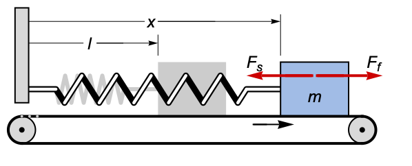
m = l = 1.;
beltv[t_] = .1;
spring[x_] = 1000.(l - x);sys := {m x''[t] == spring[x[t]] + friction[x'[t]], x[0] == 1, x'[0] == 0};
viscous[v_] := -30.(v - beltv[t]);
friction[v_] := viscous[v];{pos1, vel1} = NDSolveValue[sys, {x[t], x'[t]}, {t, 0, 2}];{Plot[{pos1}, {t, 0, 1}, PlotRange -> All], Plot[{vel1, beltv[t]}, {t, 0, 1}, PlotRange -> All]}
coulomb[v_] := -25.Sign[v - beltv[t]];
friction[v_] := viscous[v] + coulomb[v];{pos2, vel2} = NDSolveValue[sys, {x[t], x'[t]}, {t, 0, 20}];{Plot[{pos2}, {t, 0, 1}, PlotRange -> All], Plot[{vel2, beltv[t]}, {t, 0, 1}, PlotRange -> All]}![F_(str)=gamma sgn(v) e^(-2 TemplateBox[{v}, Abs])](Files/WhenEvent.zh/87.png "F_(str)=gamma sgn(v) e^(-2 TemplateBox[{v}, Abs])")
stribeck[v_] := -.3Sign[v]Exp[-2Abs[v]];
friction[v_] := viscous[v] + coulomb[v] + stribeck[v];{pos3, vel3} = NDSolveValue[sys, {x[t], x'[t]}, {t, 0, 20}];{Plot[{pos3}, {t, 0, 1}, PlotRange -> All], Plot[{vel3, beltv[t]}, {t, 0, 1}, PlotRange -> All]}静摩擦力 将方块保持在原地直至取决于表面粗糙度,弹簧力超过一定值 μ. 当方块被卡住时,使用设为 1 的离散变量 stuck,否则使用 0:
friction[v_] := viscous[v] + coulomb[v] + stribeck[v];staticsys := {x''[t] == If[stuck[t] == 1, beltv'[t], spring[x[t]] + friction[x'[t]]], x[0] == 1, x'[0] == 0};检查弹簧力是否小于 μ,并且该方块是否相对于滑动带没有移动:
μ = 100;
stick = WhenEvent[x'[t] == beltv[t], stuck[t] -> Boole[spring[x[t]]^2 < μ^2]];
slip = WhenEvent[spring[x[t]]^2 > μ^2, stuck[t] -> 0];{pos4, vel4} = NDSolveValue[{staticsys, stick, slip, stuck[0] == 0}, {x[t], x'[t]}, {t, 0, 8}, DiscreteVariables -> stuck[t]];{Plot[{pos4}, {t, 0, 2}, PlotRange -> All], Plot[{vel4, beltv[t]}, {t, 0, 2}, PlotPoints -> 100, PlotRange -> All]}Plot[{pos1, pos2, pos3, pos4}, {t, 0, 2}, PlotRange -> {0.9, 1.1}, PlotLegends -> {"viscous", "viscous+Coulomb", "viscous+Coulomb+Stribeck", "viscous+Coulomb+Stribeck+static"}]电力电子学 (4)
对由四个二极管和一个电容构成的 AC-to-DC 全波整流器建模,用于平滑输出:
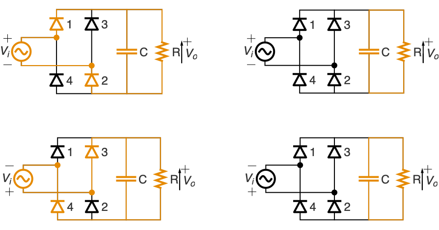
vi[t_] = Sin[t] ;vr[t_] = Abs[vi[t]]//PiecewiseExpand[#, t∈Reals]&;Plot[{vi[t], vr[t]}, {t, 0, 16}]当 vr 增加时,vo[t]=vr[t];电容器充电,并将电流供给到负载. 当 vr 开始降低 (vr'[t]<0),电容器通过负载放电,输出电压服从 vo'[t]=vo[t]/c r :
system = {vo'[t] == charging[t]vr'[t] - (1 - charging[t])vo[t] / (r c), vo[0] == 0};control = {charging[0] == 1, WhenEvent[vr'[t] < 0, charging[t] -> 0], WhenEvent[And[vo[t] < vr[t], charging[t] == 0, vr'[t] > 0], charging[t] -> 1]};pars = {r -> 0.1, c -> 1000};sol = NDSolve[{system, control} /. pars, vo, {t, 0, 16}, DiscreteVariables -> charging∈{0, 1}];Plot[{vo[t] /. sol, vr[t]}, {t, 0, 16}]对使用脉冲宽度调制反馈控制 q[t] 的 DC-to-DC 降压转换器建模,该转换器将输入电压 vi 转换到所需的输出电压 vd:
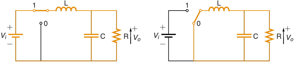
system = {vo'[t] == -vo[t] / (r c) + i[t] / c , i'[t] == -vo[t] / l + q[t]vi / l, vo[0] == 0, i[0] == 0};控制信号 q[t] 将在占每个周期 τ 的 vd/vi 时间段内接通晶体管:
control = {q[0] == 1, WhenEvent[Mod[t, τ] == (vd / vi)τ, q[t] -> 0], WhenEvent[Mod[t, τ] == 0, q[t] -> 1]};pars = {vi -> 24, vd -> 16, r -> 22, l -> 2 10 ^ -2, c -> 4 10 ^ -6, τ -> 5 10 ^ -5};sol = NDSolve[{system, control} /. pars, {vo, i, q}, {t, 0, .01}, DiscreteVariables -> q, MaxSteps -> Infinity];{Plot[{vo[t] /. sol, vd /. pars}, {t, 0, .01}, PlotRange -> All], Plot[q[t] /. sol, {t, 0, .0004}]}对使用脉冲宽度调制反馈控制 q[t] 的 DC-to-DC 升压转换器建模,该转换器将输入电压 vi 转换到所需的输出电压 vd:
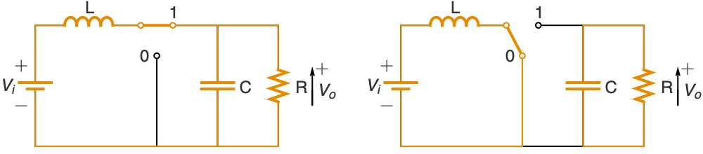
system = {vo'[t] == q[t]i[t] / c - vo[t] / (r c), i'[t] == -q[t]vo[t] / l + vi / l, vo[0] == 0, i[0] == 0};控制信号 q[t] 将在占每个周期 τ 的 vi/vd 时间段内接通晶体管:
control = {q[0] == 1, WhenEvent[Mod[t, τ] == (vi / vd)τ, q[t] -> 0], WhenEvent[Mod[t, τ] == 0, q[t] -> 1]};pars = {vi -> 24, vd -> 36, r -> 22, l -> 2 10 ^ -1, c -> 1 10 ^ -4, τ -> 5 10 ^ -5};sol = NDSolve[{system, control} /. pars, {vo, i, q}, {t, 0, .2}, DiscreteVariables -> q, MaxSteps -> Infinity];{Plot[{vo[t] /. sol, vd /. pars}, {t, 0, .2}, PlotRange -> All], Plot[q[t] /. sol, {t, 0, .0004}]}对从输入电压电平 vi 到所需输出电压电平 vo 的 DC-to-DC 升压转换器 使用脉冲宽度调制反馈控制 q[t] 建模:
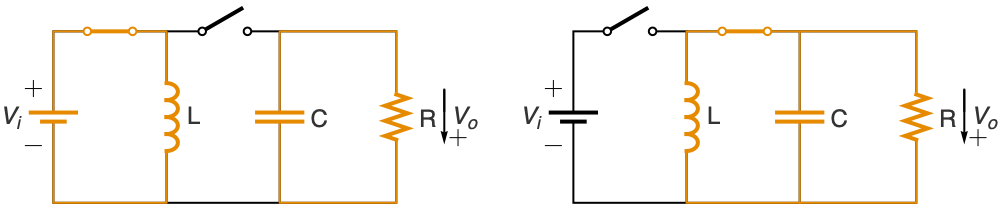
system = {i'[t] == q[t]vi / l - (1 - q[t])vo[t] / l , vo'[t] == i[t] / c - vo[t] / (r c), vo[0] == 0, i[0] == 0};控制信号 q[t] 将晶体管开启每个周期的 vd/(vi+vd) 时间:
control = {q[0] == 1, WhenEvent[Mod[t, τ] == (vd / (vd + vi))τ, q[t] -> 0], WhenEvent[Mod[t, τ] == 0, q[t] -> 1]};pars = {vi -> 24, vd -> 36, r -> 22, l -> 2 10 ^ -2, c -> 4 10 ^ -6, τ -> 5 10 ^ -5};sol = NDSolve[{system, control} /. pars, {vo, i, q}, {t, 0, .2}, DiscreteVariables -> q, MaxSteps -> Infinity];{Plot[{vo[t] /. sol, vd /. pars}, {t, 0, .02}, PlotRange -> All], Plot[q[t] /. sol, {t, 0, .0004}]}pars = {vi -> 24, vd -> 16, r -> 22, l -> 2 10 ^ -2, c -> 4 10 ^ -6, τ -> 5 10 ^ -5};sol = NDSolve[{system, control} /. pars, {vo, i, q}, {t, 0, .2}, DiscreteVariables -> q, MaxSteps -> Infinity];{Plot[{vo[t] /. sol, vd /. pars}, {t, 0, .02}, PlotRange -> All], Plot[q[t] /. sol, {t, 0, .0004}]}数字控制 (5)


system = {y'[t] == y[t] + u[t], y[0] == 1, u[0] == 0};
control = WhenEvent[Mod[t, 1.0], u[t] -> -2y[t]];NDSolve[{system, control}, {y, u}, {t, 0, 20}, DiscreteVariables -> u];Plot[Evaluate[{u[t], y[t]} /. %], {t, 0, 10}, PlotRange -> {-6, 6}]使用无振 (dead-beat) 离散时间控制器控制双重积分器:
system = {x''[t] == u[t], x[0] == 1, x'[0] == 1, u[0] == -7};
τ = 0.5;
control = WhenEvent[Mod[t, τ], u[t] -> -(1 / τ ^ 2)x[t] - (3 / (2τ))x'[t]];NDSolve[{system, control}, {x, x', u}, {t, 0, 2}, DiscreteVariables -> u];Plot[Evaluate[{x[t], x'[t], u[t]} /. %], {t, 0, 2}, PlotRange -> All]system = {x''[t] == u[t], x'[0] == x[0] == 0, u[0] == 1};kp = 1; td = 1;τ = 1; xref = 1;
control = WhenEvent[Mod[t, τ], u[t] -> kp(xref - x[t] - td x'[t])];NDSolve[{system, control}, {x, u}, {t, 0, 12}, DiscreteVariables -> u];Plot[Evaluate[{xref, x[t], u[t]} /. %], {t, 0, 12}]设计具有状态方程 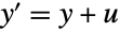 ,
, 和输出
和输出  的机械设备(plant)的离散时间控制器,仿真闭环系统:
plant = {Subscript[x, 1]'[t] == 2 Subscript[x, 1][t] + u[t], Subscript[x, 2]'[t] == 3Subscript[x, 2][t] + u[t]};pss = StateSpaceModel[plant, {Subscript[x, 1][t], Subscript[x, 2][t]}, {u[t]}, Subscript[x, 1][t] + Subscript[x, 2][t], t]ctreg = EstimatorRegulator[pss, {EstimatorGains[pss, {-12, -14}], StateFeedbackGains[pss, {-6, -7}]}]
τ = 0.0001;dtreg = ToDiscreteTimeModel[ctreg, τ, Method -> "ZeroOrderHold"]{a, b, c, d} = dtreg//Normal;controller = Sequence[WhenEvent[Mod[t, τ], {Subscript[z, 1][t], Subscript[z, 2][t], Overscript[u, ^ ][t]} ->
Evaluate@Join[a.{Subscript[z, 1][t], Subscript[z, 2][t]} + b.{u[t], Subscript[x, 1][t] + Subscript[x, 2][t]}, c.{Subscript[z, 1][t], Subscript[z, 2][t]} + d.{u[t], Subscript[x, 1][t] + Subscript[x, 2][t]}]], u[t] == -Overscript[u, ^ ][t]];init = {Subscript[x, 1][0] == 0.1, Subscript[x, 2][0] == 0.1, Subscript[z, 1][0] == 0., Subscript[z, 2][0] == 0};sol = NDSolve[{plant, controller, init}, {Subscript[x, 1], Subscript[x, 2], u}, {t, 0, 2}, DiscreteVariables -> {Overscript[u, ^ ], Subscript[z, 1], Subscript[z, 2]}];Plot[Evaluate[{Subscript[x, 1][t] + Subscript[x, 2][t], u[t]} /. sol], {t, 0, 2}, PlotRange -> All]模拟一个固定在移动车上位置为 x,角度为 θ,承受水平力为 f 的钟摆:
system = {2 f[t] + Cos[θ[t]] Derivative[1][θ][t]^2 + Sin[θ[t]] Derivative[2][θ][t] == 4 Derivative[2][x][t], 2 Cos[θ[t]] - 2 Sin[θ[t]] Derivative[2][x][t] + Derivative[2][θ][t] == 0};ssm = StateSpaceModel[system, {{x[t], 0}, {x'[t], 0}, {θ[t], (π/2)}, {θ'[t], 0}}, f[t], {}, t]gains = DiscreteLQRegulatorGains[N[ssm], {DiagonalMatrix[{1, 10, 10, 100}], {{1}}}, .1]//First利用 WhenEvent 在固定采样时间应用反馈:
control = {WhenEvent[Mod[t, .1], df[t] -> -gains.{x[t], x'[t], θ[t] - (π/2), θ'[t]}]};sol = NDSolve[Join[system /. f[t] -> df[t], control, {df[0] == 0, x[0] == x'[0] == θ'[0] == 0, θ[0] == (π/2) - 1.}], {x, θ, df}, {t, 0, 15}, DiscreteVariables -> df[t]];
Plot[Evaluate[{θ[t], df[t]} /. sol], {t, 0, 8}, PlotRange -> All]PDE 模型 (1)
模拟温控器控制下一个房间中的热生成,该房间有三面绝热墙和一面受外界温度影响的玻璃墙:
Ω = Rectangle[{0, 0}, {3 / 2, 1}];
outsideTemp[t_] := 15 + 10 * Sin[2π t / 24];
kd = 0.78;Ld = 0.05;
Γ = NeumannValue[Ld / kd * (outsideTemp[t] - u[t, x, y]), {x == 0}];
在事件发生时,加热器的负载会增大或减小. 系数 20 指定过渡的斜率:
heater[upQ_, t_, tEvent_] := Evaluate[With[{heaterLoad = 26, slope = 20}, If[upQ == 1, Min[20 * Max[(t - tEvent), 0], 1], 1 - Min[20 * Max[(t - tEvent - 1 / 8), 0], 1]] * heaterLoad]]With[{tEvent = 10},
Plot[{heater[1, t, tEvent], heater[0, t, tEvent]}, {t, 9, 11}, PlotLegends -> {"up", "down"}]]注意,up 和 down 阶段有重叠. 这可以防止它们在两种状态之间连续跳转,就像真正的控制器一样.
PDE 模拟空气中的热扩散,在圆 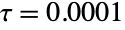 内生成热,通过玻璃窗散热:
ρ = 1.225;Cp = 1005.4;
With[{heating = heater[a[t], t, eventT[t]]},
	pde = D[u[t, x, y], t]  - ρ * Cp * Laplacian[u[t, x, y], {x, y}] == If[(x - 1 / 2) ^ 2 + (y - 1 / 2) ^ 2 ≤ (2 / 10) ^ 2, heating, 0] + Γ];
如果位于  处的温控器测量到的温度高于/低于触发温度,且离散变量
  发生变化,则关闭/打开加热器:
triggerLow = 18;triggerHigh = 20;
events = {a[0] == 1, eventT[0] == 0, WhenEvent[u[t, 1.25, .25] < triggerLow, {eventT[t], a[t]} -> {If[a[t] == 0, t, eventT[t]], 1}], WhenEvent[u[t, 1.25, .25] > triggerHigh, {eventT[t], a[t]} -> {If[a[t] == 1, t, eventT[t]], 0}]};eqn = {pde, u[0, x, y] == outsideTemp[0], events};
res = Monitor[NDSolveValue[eqn, {u, a}, {t, 0, 2 * 24}, {x, y}∈Ω, DiscreteVariables -> {eventT[t], a[t]}, EvaluationMonitor :> (monitor = Row[{"t = ", CForm[t]}])], monitor]可视化温控器测量的温度、外部温度和加热器的触发. 加热器处于开启状态时显示蓝色背景:
hp = Plot[ 25res[[2]][t], {t, 0, 2 * 24}, Filling -> Bottom, PlotStyle -> None];Show[Plot[{res[[1]][t, 1.25, .25], outsideTemp[t], 18, 20}, {t, 0, 2 * 24}], hp]查看积分过程中的时间步长,注意 NDSolveValue 如何在事件期间根据需要调整时间步长:
ListPlot[res[[1]]["Coordinates"][[1]], AxesLabel -> {"Steps", "Time"}]属性和关系 (2)
NDSolve 会尝试自动设置 WhenEvent 事件来处理 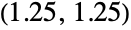 中的不连续点:
NDSolve[{x'[t] == Sign[1 - x[t]], x[0] == 2}, x, {t, 0, 2}];Plot[{x[t] /. %, x'[t] /. %}, {t, 0, 2}]NDSolve[{Derivative[1][x][t] == v[t], WhenEvent[1 == x[t], v[t] -> "DiscontinuitySignature"], x[0] == 2, v[0] == 1}, x, {t, 0, 2}, DiscreteVariables -> {Element[v, {-1, 0, 1}]}];如果  是一个黑盒(black-box)函数,NDSolve 不能自动处理不连续性:
blackbox[x_ ? NumberQ] := Sign[1 - x];NDSolve[{x'[t] == blackbox[x[t]], x[0] == 2}, x, {t, 0, 2}];
这种情况,可以通过添加 WhenEvent 正确处理不连续性:
NDSolve[{x'[t] == v[t], x[0] == 2, v[0] == 1, WhenEvent[1 == x[t], v[t] -> "DiscontinuitySignature"]}, {x, v}, {t, 0, 2}, DiscreteVariables -> {Element[v, {-1, 0, 1}]}];Plot[{x[t] /. %, x'[t] /. %}, {t, 0, 2}]或者,使用 "CrossSlidingDiscontinuity" 穿越不连续性:
NDSolve[{x'[t] == blackbox[x[t]], x[0] == 2, WhenEvent[1 - x[t], "CrossSlidingDiscontinuity"]}, x, {t, 0, 2}];Plot[{x[t] /. %, x'[t] /. %}, {t, 0, 2}]可能存在的问题 (6)
事件诠释 (1)
pred[t_ ? NumberQ, x_ ? NumberQ] := t > .5 && x > 0;
xsol = NDSolveValue[{x'[t] == 2 + x[t], x[0] == -1, WhenEvent[pred[t, x[t]], Print[{t, x[t]}]]}, x, {t, 0, 1}];
WhenEvent 不能找到显式根函数,因此当 pred 变成 True 时事件发生:
Plot[{xsol[t], Boole[pred[t, xsol[t]]]}, {t, 0, 1}]当给定显式函数 ( ),事件被认为根
  ,但条件是谓词 (
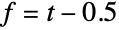 ) 在
) 在  时为 False,因此从不会被触发:
xsol = NDSolveValue[{x'[t] == 2 + x[t], x[0] == -1, WhenEvent[t > .5 && x[t] > 0, Print[{t, x[t]}]]}, x, {t, 0, 1}];显示解的踪迹和事件位置,背景为绿,当条件为 True,当条件为 False 时,背景为红色:
Show[Plot[xsol[t], {t, 0, 1}], Graphics[...]]

xsol = NDSolveValue[{x'[t] == 2 + x[t], x[0] == -1, WhenEvent[x[t] > 0 && t > .5, Print[{t, x[t]}]]}, x, {t, 0, 1}];
显示解的踪迹和事件位置,背景为绿,当条件为 True,当条件为 False 时,背景为红色:
Show[Plot[xsol[t], {t, 0, 1}], Graphics[...]]事件检测 (2)
使用默认的 "DetectionMethod",可能会错过一些事件:
NDSolve[{y'[t] == -1, y[0] == 1, WhenEvent[y[t] ^ 2 == .000001, Print[t]]}, y, {t, 0, 4}]尝试 "DerivativeSign" 或 "Interpolation" 获取更好的事件检测:
NDSolve[{y'[t] == -1, y[0] == 1, WhenEvent[y[t] ^ 2 == .000001, Print[t], "DetectionMethod" -> "DerivativeSign"]}, y, {t, 0, 4}]

NDSolve[{y'[t] == -1, y[0] == 1, WhenEvent[y[t] ^ 2 == .000001, Print[t], "DetectionMethod" -> "Interpolation"]}, y, {t, 0, 4}]

NDSolve[{y'[t] == y[t], y[0] == 1, WhenEvent[(y[t] - 2) ^ 2 == 0, Print[t]]}, y, {t, 0, 1}]NDSolve[{y'[t] == y[t], y[0] == 1, WhenEvent[(y[t] - 2) == 0, Print[t]]}, y, {t, 0, 1}]
任意接近事件 (1)
eqns = {y''[t] == -10, y[0] == 1, y'[0] == 0};
whenevent = {WhenEvent[y[t] == 0, {Sow[t], y'[t] -> -(7 / 10)y'[t]}]};
{sol, {points}} = NDSolve[Join[eqns, whenevent], y, {t, 0, 4}]//Reap;Plot[y[t] /. sol, {t, 0, 2.7}, Epilog -> {Red, Point[({#, 0}&) /@ points]}]ListPlot[RealExponent[Differences[points]]]whenevent = {WhenEvent[y[t] == 0, {Sow[t], y'[t] -> -(7 / 10)y'[t]}, "LocationMethod" -> {"Brent", AccuracyGoal -> 12, PrecisionGoal -> 12}]};{sol, {times}} = NDSolve[Join[eqns, whenevent], y, {t, 0, 4}]//Reap;ListPlot[RealExponent[Differences[times]]]zp = Last[times];mindelta = Block[{delta = zp}, While[zp + delta > zp, delta = delta / 2]; delta]whenevent = {WhenEvent[y[t] == 0, {Sow[t], y'[t] -> -(7 / 10)y'[t]}, "DetectionMethod" -> "Interpolation"]};{sol, {times}} = NDSolve[Join[eqns, whenevent], y, {t, 0, 4}]//Reap;Last[Differences[times]]mindelta = Block[{delta = 4.}, While[zp + delta > zp, delta = delta / 2]; delta];
wheneventstop = {WhenEvent[y[t] == 0, {If[t - tlast ≤ 2mindelta, tend = t;"StopIntegration", tlast = Sow[t]], y'[t] -> -(7 / 10)y'[t]}, "DetectionMethod" -> "Interpolation"]};Block[{tlast = -1}, {sol, {times}} = NDSolve[{eqns, wheneventstop}, y, {t, 0, 4}]//Reap;]
ListPlot[RealExponent[Differences[points]]]Plot[y[t] /. sol, {t, tend - 10^-12, tend}]{sol, {times}} = NDSolve[{eqns, whenevent}, y, {t, 0, 10}, WorkingPrecision -> 50]//Reap;ListPlot[RealExponent[Differences[times]]]事件行为 (2)
xsol = NDSolveValue[{x'[t] == -3x[t], x[0] == 1 / 3, WhenEvent[x[t] == 1 / 9, x'[t] -> -1]}, x, {t, 0, 2}]
Plot[{xsol[t], xsol'[t]}, {t, 0, 2}]xsol = NDSolveValue[{x'[t] == -3x[t], x[0] == 1 / 3, WhenEvent[x[t] == 1 / 9, x'[t] -> -1]}, x, {t, 0, 2}, Method -> {"EquationSimplification" -> "Residual"}]
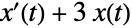
Plot[{xsol[t], xsol'[t]}, {t, 0, 2}]sol = NDSolve[{y'[t] == 0, x'[t] == 0, x[0] == 1, y[0] == 2, WhenEvent[t == .5, {x[t] -> y[t], y[t] -> x[t]}]}, {x, y}, {t, 0, 1}];Plot[Evaluate[{x[t], y[t]} /. sol], {t, 0, 1}, PlotRange -> All, PlotStyle -> {Blue, Red}, AxesOrigin -> {0, 0}]sol = NDSolve[{y'[t] == 0, x'[t] == 0, x[0] == 1, y[0] == 2, WhenEvent[t == .5, {x[t], y[t]} -> {y[t], x[t]}]}, {x, y}, {t, 0, 1}];Plot[Evaluate[{x[t], y[t]} /. sol], {t, 0, 1}, PlotRange -> All, PlotStyle -> {Blue, Red}, AxesOrigin -> {0, 0}]互动范例 (2)
ball2d[r_ ? NumericQ] := NDSolveValue[{
	x'[t] == vx[t], WhenEvent[x[t] ^ 2 == 1, vx[t] -> -vx[t]],
	y'[t] == vy[t], WhenEvent[y[t] ^ 2 == 1, vy[t] -> -vy[t]],
	x[0] == 0, y[0] == 0, vx[0] == 1, vy[0] == r
}, {x[t], y[t]}, {t, 0, 200}, DiscreteVariables -> {vx, vy}];{sol1, sol2} = {ball2d[4 / 3], ball2d[Sqrt[2]]};Manipulate[
GraphicsRow[ParametricPlot[#, {t, 0, τ}, Frame -> True, FrameTicks -> None, PlotRange -> 1, Axes -> False, PlotPoints -> 500, PlotStyle -> Thickness[0.02], Epilog -> {PointSize[.05], Point[# /. (t -> τ)]}]& /@ {sol1, sol2}], {{τ, 11.9}, 0.01, 198}, SaveDefinitions -> True]ball3d[r1_ ? NumericQ, r2_ ? NumericQ] := NDSolveValue[{x'[t] == a[t], y'[t] == b[t], z'[t] == c[t], x[0] == 0, y[0] == 0, z[0] == 0, a[0] == 1, b[0] == r1, c[0] == r2, WhenEvent[x[t] ^ 2 - 1, a[t] -> -a[t]], WhenEvent[y[t] ^ 2 - 1, b[t] -> -b[t]], WhenEvent[z[t] ^ 2 - 1, c[t] -> -c[t]]}, {x[t], y[t], z[t]}, {t, 0, 200}, DiscreteVariables -> {a, b, c}];{sol1, sol2} = {ball3d[1 / 3, 2 / 3], ball3d[Sqrt[2], Sqrt[3]]};Manipulate[
GraphicsRow[Show[ParametricPlot3D[#, {t, 0, τ}, Boxed -> True, PlotRange -> 1, Axes -> False, PlotPoints -> 500], Graphics3D[{Blue, Sphere[# /. (t -> τ), 1 / 8] /. (t -> τ)}]]& /@ {sol1, sol2}], {{τ, 11.5}, 0.01, 200, 1}, SaveDefinitions -> True]文本
Wolfram Research (2012),WhenEvent,Wolfram 语言函数,https://reference.wolfram.com/language/ref/WhenEvent.html (更新于 2014 年).
CMS
Wolfram 语言. 2012. "WhenEvent." Wolfram 语言与系统参考资料中心. Wolfram Research. 最新版本 2014. https://reference.wolfram.com/language/ref/WhenEvent.html.
APA
Wolfram 语言. (2012). WhenEvent. Wolfram 语言与系统参考资料中心. 追溯自 https://reference.wolfram.com/language/ref/WhenEvent.html 年