

HyperbolicDistribution
HyperbolicDistribution[α,β,δ,μ]
represents a hyperbolic distribution with location parameter μ, scale parameter δ, shape parameter α, and skewness parameter β.
HyperbolicDistribution[λ,α,β,δ,μ]
represents a generalized hyperbolic distribution with shape parameter λ.
Details
- The probability density for value
 in a hyperbolic distribution is proportional to
  .
. - The probability density for value
 in a generalized hyperbolic distribution is proportional to
 ![ⅇ^(beta (x-mu))sqrt(delta^2+(x-mu)^2)^(lambda-1/2) TemplateBox[{{lambda, -, {1, /, 2}}, {alpha, , {sqrt(, {{delta, ^, 2}, +, {{(, {x, -, mu}, )}, ^, 2}}, )}}}, BesselK]](Files/HyperbolicDistribution.en/4.png "ⅇ^(beta (x-mu))sqrt(delta^2+(x-mu)^2)^(lambda-1/2) TemplateBox[{{lambda, -, {1, /, 2}}, {alpha, , {sqrt(, {{delta, ^, 2}, +, {{(, {x, -, mu}, )}, ^, 2}}, )}}}, BesselK]") .
. - HyperbolicDistribution allows α and δ to be any positive real number, λ and μ any real number, and β such that
 .
. - HyperbolicDistribution allows α and β to be any quantities of the same unit dimensions, and μ, δ, λ to be quantities such that α μ, α δ, and λ are dimensionless. »
- HyperbolicDistribution can be used with such functions as Mean, CDF, and RandomVariate.
Background & Context
- HyperbolicDistribution[λ,α,β,δ,μ] represents a continuous statistical distribution defined on the set of real numbers and parametrized by positive real numbers α (a "shape parameter") and δ (a "scale parameter") and real numbers λ (a second "shape parameter"), μ (a "location parameter"), and β (a "skewness parameter"), which satisfies
 . Overall, the probability density function (PDF) of a hyperbolic distribution is smooth and unimodal, though the specific properties of the PDF graph (i.e. horizontal position, height, steepness, and concavity) are determined by the values taken on by its various parameters. It is worth noting that the so-called shape parameters δ and λ have distinct but similar effects on the shape of the PDF and combine to determine the concentration of the graph of the PDF around its peak, as well as the "closeness" of the PDF to the
  axis. In addition, the tails of the PDF of a hyperbolic distribution are "semi-heavy", in the sense that the PDF decreases exponentially for large values of
  but decreases more slowly than a Gaussian distribution (see NormalDistribution). The five-parameter version of HyperbolicDistribution is sometimes referred to as the generalized hyperbolic distribution, while the four-parameter incarnation HyperbolicDistribution[α,β,δ,μ] is equivalent to HyperbolicDistribution[1,α,β,δ,μ] and is often referred to as "the" hyperbolic distribution.
 - The theoretical roots of hyperbolic distributions date to the early 1940s and the work of British polymath R. A. Bagnold. However, their firm establishment as probability distributions occurred only some 35 years later (in the late 1970s) as part of the work of Danish statistician Ole Barndorff-Nielsen. Hyperbolic distributions are characterized by the fact that the logarithms of their PDFs are hyperbolas. Hyperbolic distributions have been used extensively in probability to approximate theoretical distributions that are unknown, with the exception of certain qualitative information. Among the most fundamental real-world uses of hyperbolic and generalized hypergeometric distributions are in the area of finance, where they have been used to model financial and stock returns, price movements, portfolio risk, and general market behavior. Hyperbolic distributions have also been used to measure turbulent wind speeds and the movement of wind-blown sand.
- RandomVariate can be used to give one or more machine- or arbitrary-precision (the latter via the WorkingPrecision option) pseudorandom variates from a hyperbolic distribution. Distributed[x,HyperbolicDistribution[λ,α,β,δ,μ]], written more concisely as xHyperbolicDistribution[λ,α,β,δ,μ], can be used to assert that a random variable x is distributed according to a hyperbolic distribution. Such an assertion can then be used in functions such as Probability, NProbability, Expectation, and NExpectation.
- The probability density and cumulative distribution functions may be given using PDF[HyperbolicDistribution[λ,α,β,δ,μ],x] and CDF[HyperbolicDistribution[λ,α,β,δ,μ],x]. The mean, median, variance, raw moments, and central moments may be computed using Mean, Median, Variance, Moment, and CentralMoment, respectively.
- DistributionFitTest can be used to test if a given dataset is consistent with a hyperbolic distribution, EstimatedDistribution to estimate a hyperbolic parametric distribution from given data, and FindDistributionParameters to fit data to a hyperbolic distribution. ProbabilityPlot can be used to generate a plot of the CDF of given data against the CDF of a symbolic hyperbolic distribution, and QuantilePlot to generate a plot of the quantiles of given data against the quantiles of a symbolic hyperbolic distribution.
- TransformedDistribution can be used to represent a transformed hyperbolic distribution, CensoredDistribution to represent the distribution of values censored between upper and lower values, and TruncatedDistribution to represent the distribution of values truncated between upper and lower values. CopulaDistribution can be used to build higher-dimensional distributions that contain a hyperbolic distribution, and ProductDistribution can be used to compute a joint distribution with independent component distributions involving hyperbolic distributions.
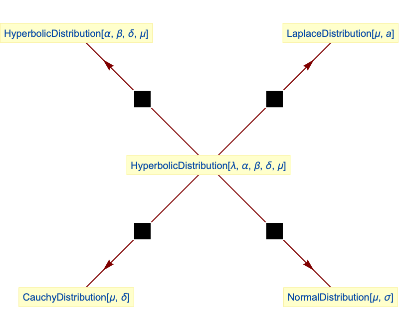
- HyperbolicDistribution is closely related to a number of other distributions. For example, because of its generality, HyperbolicDistribution includes distributions such as LaplaceDistribution, StudentTDistribution, NormalDistribution, InverseGaussianDistribution, GammaDistribution, VarianceGammaDistribution, and CauchyDistribution as either special or limiting cases. The generalized HyperbolicDistribution can also be viewed as a parameter mixture (see ParameterMixtureDistribution) of NormalDistribution and InverseGaussianDistribution, in the sense that the PDF of HyperbolicDistribution[λ,α,β,δ,μ] is precisely the same as that of ParameterMixtureDistribution[NormalDistribution[μ+β u,
 ],u InverseGaussianDistribution[δ/
 ,δ2,λ]]. HyperbolicDistribution is also related to ChiDistribution, ChiSquareDistribution, FRatioDistribution, and HalfNormalDistribution.
Examples
open all close allBasic Examples (3)
Probability density function of a hyperbolic distribution:
Plot[Table[PDF[HyperbolicDistribution[2, β, 3, 1], x], {β, {-1.5, 0, 1}}]//Evaluate, {x, -8, 8}, Exclusions -> None, Filling -> Axis]Plot[Table[PDF[HyperbolicDistribution[α, 1.5, 3, 1], x], {α, {2, 3, 4}}]//Evaluate, {x, 0, 10}, Exclusions -> None, Filling -> Axis]PDF[HyperbolicDistribution[α, β, δ, μ], x]Cumulative distribution function of a hyperbolic distribution:
Plot[Table[CDF[HyperbolicDistribution[2, β, 3, 1], x], {β, {-1.5, 0, 1}}]//Evaluate, {x, -8, 8}, Filling -> Axis]Plot[Table[CDF[HyperbolicDistribution[α, 1.5, 3, 1], x], {α, {2, 3, 4}}]//Evaluate, {x, 0, 10}, Filling -> Axis]Mean and variance of a hyperbolic distribution:
Mean[HyperbolicDistribution[α, β, δ, μ]]Variance[HyperbolicDistribution[α, β, δ, μ]]Scope (14)
Probability density function of a generalized hyperbolic distribution:
Plot[Table[PDF[HyperbolicDistribution[λ, 2, 1.5, 3, 1], x], {λ, {-2, 0, 1.5}}]//Evaluate, {x, 0, 10}, Filling -> Axis, Exclusions -> None]PDF[HyperbolicDistribution[λ, α, β, δ, μ], x]Cumulative distribution function of a generalized hyperbolic distribution:
Plot[Table[CDF[HyperbolicDistribution[λ, 2, 1.5, 3, 1], x], {λ, {-2, 0, 1.5}}]//Evaluate, {x, 0, 10}, Filling -> Axis]Mean and variance of a generalized hyperbolic distribution:
Mean[HyperbolicDistribution[λ, α, β, δ, μ]]Variance[HyperbolicDistribution[λ, α, β, δ, μ]]Generate a sample of pseudorandom numbers from a hyperbolic distribution:
sample = RandomVariate[HyperbolicDistribution[2, 1.5, 3, 0], 10 ^ 5];Compare its histogram to the PDF:
Show[
	Histogram[sample, {-5, 20, 1}, "PDF"],
	Plot[PDF[HyperbolicDistribution[2, 1.5, 3, 0], x], {x, -5, 15}, PlotStyle -> Thick]]
Distribution parameters estimation:
sample = RandomVariate[HyperbolicDistribution[4, 1, 3, 3], 10 ^ 3];Estimate the distribution parameters from sample data:
edist = EstimatedDistribution[sample, HyperbolicDistribution[α, 1, δ, γ]]Compare the density histogram of the sample with the PDF of the estimated distribution:
Show[Histogram[sample, Automatic, "PDF"], Plot[PDF[edist, x], {x, -1, 7}, PlotStyle -> Thick]]Skewness of a hyperbolic distribution:
Plot3D[Skewness[HyperbolicDistribution[α, β, 2, 0]], {α, 4, 8}, {β, -3, 3}, MeshFunctions -> {#3&}, MeshShading -> ColorData[35, "ColorList"], AxesLabel -> Automatic]Of a generalized hyperbolic distribution:
Plot3D[Skewness[HyperbolicDistribution[λ, 3, β, 2, 0]]//Evaluate, {λ, -3, 3}, {β, -3, 3}, MeshFunctions -> {#3&}, MeshShading -> ColorData[35, "ColorList"], AxesLabel -> Automatic]Kurtosis of a hyperbolic distribution:
Plot3D[Kurtosis[HyperbolicDistribution[α, β, 2, 0]], {α, 4, 8}, {β, -3, 3}, MeshFunctions -> {#3&}, MeshShading -> ColorData[35, "ColorList"], AxesLabel -> Automatic]Of a generalized hyperbolic distribution:
Plot3D[Kurtosis[HyperbolicDistribution[λ, 3, β, 2, 0]]//Evaluate, {λ, -3, 3}, {β, -3, 3}, MeshFunctions -> {#3&}, MeshShading -> ColorData[35, "ColorList"], AxesLabel -> Automatic]Different moments with closed forms as functions of parameters for hyperbolic distribution:
FormulaGrid[list_, type_] := Grid[...]FormulaGrid[Table[Moment[HyperbolicDistribution[α, β, δ, μ], r], {r, 3}], M]FormulaGrid[Table[CentralMoment[HyperbolicDistribution[α, β, δ, μ], r], {r, 3}], CM]FormulaGrid[Table[FactorialMoment[HyperbolicDistribution[α, β, δ, μ], r], {r, 3}], FM]FormulaGrid[Table[Cumulant[HyperbolicDistribution[α, β, δ, μ], r], {r, 3}], C]Different moments with closed forms as functions of parameters for generalized hyperbolic distribution:
FormulaGrid[list_, type_] := Grid[...]FormulaGrid[Table[Moment[HyperbolicDistribution[λ, α, β, δ, μ], r], {r, 3}], M]FormulaGrid[Table[CentralMoment[HyperbolicDistribution[λ, α, β, δ, μ], r], {r, 3}], CM]FormulaGrid[Table[FactorialMoment[HyperbolicDistribution[λ, α, β, δ, μ], r], {r, 3}], FM]FormulaGrid[Table[Cumulant[HyperbolicDistribution[λ, α, β, δ, μ], r], {r, 3}], C]Hazard function of a hyperbolic distribution:
Plot[Table[HazardFunction[HyperbolicDistribution[α, 0.3, 2, -2], x], {α, {0.5, 1, 2}}]//Evaluate, {x, -5, 5}, Filling -> Axis]Plot[Table[HazardFunction[HyperbolicDistribution[3, β, 2, -2], x], {β, {0.5, 1, 2}}]//Evaluate, {x, -5, 5}, Filling -> Axis]Hazard function of a generalized hyperbolic distribution:
Plot[Table[HazardFunction[HyperbolicDistribution[λ, 2, 0.3, 2, -2], x], {λ, {-1.5, 1, 3}}]//Evaluate, {x, -5, 5}, Filling -> Axis]Quantile function of a hyperbolic distribution:
Plot[Table[Quantile[HyperbolicDistribution[α, 0.3, 2, -2], q], {α, {0.5, 1, 4}}]//Evaluate, {q, 0, 1}, Filling -> Axis]Plot[Table[Quantile[HyperbolicDistribution[10, β, 2, -2], q], {β, {0.5, 3, 8}}]//Evaluate, {q, 0, 1}, Filling -> Axis]Quantile function of a generalized hyperbolic distribution:
Plot[Table[Quantile[HyperbolicDistribution[λ, 2, 0.3, 2, -2], q], {λ, {-1.5, 3, 6}}]//Evaluate, {q, 0, 1}, Filling -> Axis]Consistent use of Quantity in parameters yields QuantityDistribution:
pos𝒟 = HyperbolicDistribution[Quantity[2.865, 1/"Millimeters"], Quantity[0.745, 1/"Millimeters"], Quantity[1.3, "Millimeters"], Quantity[-0.54, "Millimeters"]];Mean[pos𝒟]Applications (5)
A logarithm of the diameter (in millimeters) of mined diamonds follows HyperbolicDistribution with parameters ![]() ,
, ![]() ,
, ![]() , and
, and ![]() :
:
diamonSize𝒟 = HyperbolicDistribution[2.865, 0.745, 1.3, -0.54];ls = RandomVariate[diamonSize𝒟, 10 ^ 5];Show[Histogram[ls, 25, "PDF"], Plot[PDF[diamonSize𝒟, x], {x, Min[ls], Max[ls]}, PlotStyle -> Thick]]Find the probability that the diamond's diameter exceeds 5 millimeters:
NProbability[Exp[x] > 5, xdiamonSize𝒟]Normal inverse Gaussian (NIG) distribution is a special case of HyperbolicDistribution:
NIGdist = HyperbolicDistribution[-1 / 2, α, β, δ, μ];It has a particularly simple moment-generating function:
MomentGeneratingFunction[NIGdist, t]Hence the sum of NIG variates also follows NIG distribution:
TransformedDistribution[Subscript[x, 1] + Subscript[x, 2], {Subscript[x, 1]HyperbolicDistribution[-1 / 2, α, β, Subscript[δ, 1], Subscript[μ, 1]], Subscript[x, 2]HyperbolicDistribution[-1 / 2, α, β, Subscript[δ, 2], Subscript[μ, 2]]}]Fit the daily logarithmic return of the S&P 500 index since 2005 to NIG distribution:
data = Differences[Log@FinancialData["SP500", "Close", "Jan 1., 2005", "Value"]];dist = EstimatedDistribution[data, HyperbolicDistribution[-1 / 2, α, β, δ, μ]]Compare the density of the estimated distribution to a data histogram:
Show[Histogram[data, Automatic, "PDF"], Plot[PDF[dist, x], {x, -.5, .5}, PlotRange -> All, PlotStyle -> Thick]]Variance-gamma distribution (see this Demonstration) is the limiting case of ![]() for
for ![]() :
:
pdf = PDF[HyperbolicDistribution[λ, α, β, δ, μ], x];assumps = λ > 0 && α > 0 && -α < β < α && {x, μ}∈Reals;Find the limiting probability density function:
pdf = Assuming[assumps, Limit[Series[pdf, {δ, 0, 1}], δ -> 0, Direction -> -1]]Compare with the PDF of the built-in VarianceGammaDistribution:
FullSimplify[pdf == PDF[VarianceGammaDistribution[λ, α, β, μ], x], x > μ && assumps]FullSimplify[pdf == PDF[VarianceGammaDistribution[λ, α, β, μ], x], x < μ && assumps]Compare the histogram of the variance-gamma distribution to its PDF:
Block[{α = 2, β = 1, μ = 0, λ = 1},
	Show[Histogram[RandomVariate[VarianceGammaDistribution[λ, α, β, μ], 10 ^ 4], 25, "PDF"], Plot[pdf, {x, -3, 6}, PlotRange -> All, PlotStyle -> Thick]]]
Generalized hyperbolic (GH) skew ![]() distribution is obtained in the limit of
distribution is obtained in the limit of ![]() :
:
pdf = PDF[HyperbolicDistribution[-ν / 2, Sqrt[β^2 + ϵ], β, Sqrt[ν], μ], x];
assumps = ν > 0 && {x, μ}∈Reals && β^2 > 0;
Find the limiting probability density function:
pdf = Assuming[assumps, Limit[Series[pdf, {ϵ, 0, 1}], ϵ -> 0, Direction -> -1]]The GH skew ![]() distribution also admits parameter mixture representation:
distribution also admits parameter mixture representation:
ghSkewTdist = ParameterMixtureDistribution[NormalDistribution[μ + β u, Sqrt[u]], uInverseGammaDistribution[ν / 2, ν / 2]];Refine[PDF[ghSkewTdist, x], assumps]Check that densities are equal:
FullSimplify[% / pdf, assumps]Compare the histogram of the variance-gamma distribution to its PDF:
Block[{β = 1, μ = 0, λ = 1, ν = 9},
	Show[Histogram[RandomVariate[ghSkewTdist, 10 ^ 4], 25, "PDF"], Plot[pdf, {x, -3, 6}, PlotRange -> All, PlotStyle -> Thick]]]
Student ![]() distribution corresponds to
distribution corresponds to ![]() :
:
PDF[ghSkewTdist /. β -> 0, x]The logarithm of population of towns, cities, and villages in the United States can be modeled by HyperbolicDistribution:
popdata = CityData[#, "Population"]& /@ CityData[{All, "UnitedStates"}];Remove missing and zero values:
cleandata = Select[DeleteMissing[popdata], Positive]//N;Data histogram on the log-log scale:
Histogram[cleandata, {"Log", "Sturges"}, "LogPDF", AxesLabel -> Automatic]Fit the population logarithm to HyperbolicDistribution:
logdata = Log10[QuantityMagnitude[cleandata]];hd = EstimatedDistribution[logdata, HyperbolicDistribution[a, b, c, d]]Compare the data histogram to the fitted density plot:
Show[Histogram[logdata, 25, "PDF", Ticks -> {Table[{k, With[{kk = k}, HoldForm[10 ^ kk]], {0, .02}, Thick}, {k, {1, 2, 4, 6}}], Automatic}], Plot[PDF[hd, x], {x, 0, 7}, PlotStyle -> Thick]]Properties & Relations (9)
Hyperbolic distribution is closed under translation and scaling:
TransformedDistribution[a * u + b, uHyperbolicDistribution[α, β, δ, μ]]Hyperbolic distribution is closed under addition under some assumptions:
TransformedDistribution[Subsuperscript[∑, i = 1, 3]Subscript[x, i], Table[Subscript[x, i]HyperbolicDistribution[-1 / 2, α, β, Subscript[δ, i], Subscript[μ, i]], {i, 3}]]The logarithm of the PDF of a hyperbolic distribution is a hyperbola:
With[{β = .3, δ = 1.5, μ = 4, α = 1}, Log[PDF[HyperbolicDistribution[α, β, δ, μ], x]^2]]PowerExpand[%]With[{β = .3, δ = 1.5, μ = 4}, Plot[Table[-Log[PDF[HyperbolicDistribution[α, β, δ, μ], x]], {α, r = {0.5, 1, 2, 4}}]//Evaluate, {x, -5, 13}, PlotLegends -> (Row[{"α = ", #}]& /@ r)]]The logarithm of the PDF can be written as a general hyperbola equation ![]() with determinant condition
with determinant condition ![]() :
:
y - Log[PDF[HyperbolicDistribution[α, β, δ, μ], x]] /. (Sqrt[α^2 - β^2]/2 α δ BesselK[1, Sqrt[α^2 - β^2] δ]) -> const//FullSimplify[#, x∈Reals && -α < β < α && δ > 0 && μ∈Reals]&(% - α Sqrt[δ^2 + (x - μ)^2])^2 - (α Sqrt[δ^2 + (x - μ)^2])^2//Expand//Collect[#, {x, y, x y}]&The determinant condition is satisfied:
Det[{{ (-α^2 + β^2), -β}, {-β, 1}}]Relationships to other distributions:
Generalized hyperbolic distribution simplifies to hyperbolic distribution:
PDF[HyperbolicDistribution[1, α, β, δ, μ], x]//FullSimplify[#, α > 0]&PDF[HyperbolicDistribution[α, β, δ, μ], x]% - %%//FullSimplify[#, δ > 0 && -α < β < α && α > 0]&Generalized hyperbolic distribution is a transformation of NormalDistribution and InverseGaussianDistribution:
TransformedDistribution[μ + β u + Sqrt[u] z, {z NormalDistribution[], uInverseGaussianDistribution[δ / Sqrt[α ^ 2 - β ^ 2], δ ^ 2, λ]}]It can also be interpreted as ParameterMixtureDistribution:
𝒟 = ParameterMixtureDistribution[NormalDistribution[μ + β u, Sqrt[u]], uInverseGaussianDistribution[δ / Sqrt[α ^ 2 - β ^ 2], δ ^ 2, λ]];PDF[𝒟, x]//PowerExpand//Simplify[#, α > 0]&PDF[HyperbolicDistribution[λ, α, β, δ, μ], x]//PowerExpandFullSimplify[% - %%, α > 0 && δ > 0 && -α < β < α]CauchyDistribution is a singular limit of ![]() , given
, given ![]() and
and ![]() :
:
Limit[PDF[HyperbolicDistribution[-1 / 2, α, 0, δ, μ], x], α -> 0]//FullSimplifyPDF[CauchyDistribution[μ, δ], x]FullSimplify[% - %%]NormalDistribution is the limiting case of ![]() for
for ![]() and
and ![]() :
:
Limit[With[{β = 0, δ = σ^2α}, PDF[HyperbolicDistribution[λ, α, β, δ, μ], x]], α -> Infinity, Assumptions -> σ > 0 && {λ, μ, x}∈Reals]PDF[NormalDistribution[μ, σ], x]% - %%LaplaceDistribution is the limiting case of ![]() when
when ![]() and
and ![]() :
:
Limit[PDF[HyperbolicDistribution[α, 0, δ, μ], x], δ -> 0]PDF[LaplaceDistribution[μ, 1 / α], x]FullSimplify[%% - %, {x, μ}∈Reals]Neat Examples (1)
PDFs for different β values with CDF contours:
dist = HyperbolicDistribution[2.3, β, 3, 1];cdf = Function[{x, β}, Evaluate[CDF[dist, x]]];
ql = {0.025, 0.10, 0.25, 0.5, 0.75, 0.90, 0.975};
cl = Table[ColorData["Rainbow"][q], {q, Join[{0.0}, ql]}];Legended[Plot3D[PDF[dist, x], {x, -10, 5}, {β, -2, 2}, PlotTheme -> "Marketing", MeshFunctions -> {cdf}, Mesh -> {ql}, MeshStyle -> GrayLevel[0.8], MeshShading -> cl, AxesLabel -> Automatic, BaseStyle -> Opacity[0.9], ImageSize -> 400, PlotPoints -> 60], BarLegend["Rainbow", ql, LegendLabel -> "prob"]]Text
Wolfram Research (2010), HyperbolicDistribution, Wolfram Language function, https://reference.wolfram.com/language/ref/HyperbolicDistribution.html (updated 2016).
CMS
Wolfram Language. 2010. "HyperbolicDistribution." Wolfram Language & System Documentation Center. Wolfram Research. Last Modified 2016. https://reference.wolfram.com/language/ref/HyperbolicDistribution.html.
APA
Wolfram Language. (2010). HyperbolicDistribution. Wolfram Language & System Documentation Center. Retrieved from https://reference.wolfram.com/language/ref/HyperbolicDistribution.html