



NDSolve
NDSolve[eqns,u,{x,xmin,xmax}]
xminから xmaxの範囲における独立変数 x の関数 u について,常微分方程式 eqns の数値解を求める.
NDSolve[eqns,u,{x,xmin,xmax},{y,ymin,ymax}]
偏微分方程式 eqns を矩形領域上で解く.
NDSolve[eqns,u,{x,y}∈Ω]
偏微分方程式 eqns を,領域 Ω 上で解く.
NDSolve[eqns,u,{t,tmin,tmax},{x,y}∈Ω]
時間依存偏微分方程式 eqns を,領域 Ω 上で解く.
NDSolve[eqns,{u1,u2,…},…]
関数 uiを解く.
詳細とオプション
- NDSolveは,結果をInterpolatingFunctionオブジェクトで与える数値微分方程式ソルバである.
- NDSolve[eqns,u[x],{x,xmin,xmax}]は,関数 u 自体の解を与える代りに u[x]の解を与える.
- 微分方程式は,Dtで得られる全微分商ではなく,Dで得られる u'[x]のような導関数で記述しなければならない.
- 偏微分方程式は,微分演算子のGrad (∇),Div (∇.),Laplacian (∇2),Curl (∇)を使って指定することもできる.一般に,これらの演算子は,演算子形が評価されるのを防ぐために,Inactive[op]で使われる.
- NDSolveは,多種の常微分方程式と多くの偏微分方程式を解くことができる.
- NDSolveは,多くの遅延微分方程式も解くことができる.
- 常微分方程式では,関数 uiは単一変数 t だけに依存するものとする.偏微分方程式では,複数の変数に依存してもよい.
- WhenEvent[event,action]を方程式 eqns に入れて event がTrueになったときに実現する action を指定することができる.
- uiの完全解を得るには,十分な初期条件または境界条件を微分方程式に与えておかなければならない.
- 初期条件と境界条件は,通常 u[x0]==c0, u'[x0]==dc0のように与える.実際に与える式はより複雑なものであっても構わない.
- c0,dc0等は,u[x]がベクトルあるいは一般的なリストの値を持つ関数であることを指定するリストでもよい.
- 周期境界条件は u[x0]==u[x1]を用いて指定することができる.
- 初期条件や境界条件に現れる点 x0は,解を求める xminから xmaxの範囲に必ずしもなくてよい.
- 境界値もまたDirichletConditionおよびNeumannValue.を使って指定することができる.
- 遅延微分方程式では,最初の履歴関数が u[x/;x<x0]==c0の形式で与えられる.ただし,c0は一般に x の関数である.
- NDSolveの微分方程式には,複素数を使うことができる.
- NDSolveは多くの微分代数方程式を解くことができる.この場合,eqns が純粋に代数的なこともあれば,変数のあるものが陰的に代数的なこともある.
- uiは従属変数の関数であり得るが,そのような変数すべてを含んでいる必要はない.
- 指定可能なオプション
-
AccuracyGoal Automatic 目標とする絶対確度の桁数 Compiled Automatic 式を自動的にコンパイルするかどうか DependentVariables Automatic 全従属変数のリスト EvaluationMonitor None 関数が評価されたときに常に評価される式 InitialSeeding {} いくつかのアルゴリズムのためのシード方程式 InterpolationOrder Automatic 最終出力の連続性の程度 MaxStepFraction 1/10 各ステップでカバーする領域の最大割合 MaxSteps Automatic 最大ステップ数 MaxStepSize Automatic 各ステップの最大刻み幅 Method Automatic 使用されるアルゴリズム NormFunction Automatic 誤差推定に用いるノルム PrecisionGoal Automatic 目標とする精度の桁数 StartingStepSize Automatic 使用する最初の刻み幅 StepMonitor None ステップを取る際に評価される式 WorkingPrecision MachinePrecision 内部計算で使用する精度 - NDSolveは解における推定誤差がPrecisionGoalとAccuracyGoalで指定された許容率内に収まるような刻み幅を取る.
- オプションNormFunction->f は各 uiの推定誤差を f[{e1,e2,…}]を用いて統合するように指定する.
- AccuracyGoalは,実質的に解を求める各ステップで許される絶対的な局所誤差を指定し,PrecisionGoalは相対的な局所誤差を指定する.
- 解がゼロ近傍にあるときに,解が正確に求められなければならない場合は,AccuracyGoalを大き目に設定するか,Infinityに設定するとよい.
- AccuracyGoalやPrecisionGoalのデフォルト値のAutomaticはWorkingPrecision/2に等しい.
- MaxStepsのデフォルト設定Automaticは,開始時および終了時と推定されるステップサイズによるNDSolveの最大ステップ数を推定している.これが不可能な場合には,固定ステップ数が使われる.
- MaxStepFractionの設定で各独立変数の値の幅の割合としてNDSolveの最大刻み幅を指定する.
- DependentVariables->Automaticの場合,NDSolveは与えられた方程式を解析して従属変数を決定しようとする.
- NDSolveは一般に微分方程式を,その方程式のタイプによっていくつかの異なるステージに分けて解く.Method->{s1->m1,s2->m2,…}では,ステージ si がメソッド miによって処理される.実際に使われるステージとその順序は,解こうとしている問題に基づいてNDSolveによって決定される.
- 使用可能な解法のステージ
-
"TimeIntegration" 微分方程式系の時間積分 "BoundaryValues" 常微分方程式の境界値解 "DiscontinuityProcessing" 不連続微分方程式を扱うための記号処理 "EquationSimplification" 数値評価のための方程式形式の簡略 "IndexReduction" 微分代数方程式の記号指数簡約 "DAEInitialization" 微分代数方程式の一貫した初期化 "PDEDiscretization" 偏微分方程式の離散化 - Method->m1 またはMethod->{m1,s2->m2,…}を使うと,メソッド m1は時間積分に使われると仮定されるので,Method->m1 はMethod->{"TimeIntegration"->m1}に等しい.
- Methodオプションの可能な明示的時間積分設定
-
"Adams" 一次から12次の予測器・修正子Adams法 "BDF" 一次から五次の陰的後退微分法 "ExplicitRungeKutta" 二次あるいは一次から九次あるいは八次のルンゲ・クッタ法の適応的埋込み型ペア "IDA" 微分代数方程式の陰的後退微分公式 "ImplicitRungeKutta" 任意次数の陰的ルンゲ・クッタ法の族 "SymplecticPartitionedRungeKutta" 分離可能なハミルトン系のためのインターリーブ・ルンゲ・クッタ法 - Method->{"controller",Method->"submethod"}あるいはMethod->{"controller",Method->{m1,m2,…}}のときの可能なコントローラ法
-
"Composition" サブメソッドのリストを作成 "DoubleStep" ダブルステップ法による刻み幅を適用 "EventLocator" 指定事象に応答 "Extrapolation" 多項式補外を用いて次数と刻み幅を適用 "FixedStep" 固定刻み幅を使用 "OrthogonalProjection" 直交制約条件を満たす解を投影 "Projection" 一般的な制約条件を満足する解を投影 "Splitting" 式を分割し異なるサブメソッドを使用 "StiffnessSwitching" 硬さが検出されたら陽的メソッドから陰的メソッドに変更 - 主にサブメソッドとして使われるメソッド
-
"ExplicitEuler" 前進オイラー法 "ExplicitMidpoint" 中点法則法 "ExplicitModifiedMidpoint" Graggの補整を伴う中点法則法 "LinearlyImplicitEuler" 線形陰的オイラー法 "LinearlyImplicitMidpoint" 線形陰的中点法則法 "LinearlyImplicitModifiedMidpoint" 線形陰的Bader補整中点法則法 "LocallyExact" 局所的に厳密な記号解の数値近似 - InterpolationOrder->Allと設定すると,NDSolveはもとになるメソッドと同じ次数の補間を使う解を生成するようになる. »
例題
すべて開く すべて閉じる例 (7)
s = NDSolve[{y'[x] == y[x]Cos[x + y[x]], y[0] == 1}, y, {x, 0, 30}]Plot[Evaluate[y[x] /. s], {x, 0, 30}, PlotRange -> All]ParametricPlot[Evaluate[{y[x], y'[x]} /. s], {x, 0, 20}]{y[10.5], y'[12.5]} /. ss = NDSolve[{y''[x] + Sin[y[x]]y[x] == 0, y[0] == 1, y'[0] == 0}, y, {x, 0, 30}]Plot[Evaluate[{y[x], y'[x], y''[x]} /. s], {x, 0, 30}, PlotStyle -> Automatic]s = NDSolve[{x'[t] == -y[t] - x[t] ^ 2, y'[t] == 2x[t] - y[t] ^ 3, x[0] == y[0] == 1}, {x, y}, {t, 20}]ParametricPlot[Evaluate[{x[t], y[t]} /. s], {t, 0, 20}]NDSolve[{D[u[t, x], t] == D[u[t, x], x, x], u[0, x] == 0, u[t, 0] == Sin[t], u[t, 5] == 0}, u, {t, 0, 10}, {x, 0, 5}]Plot3D[Evaluate[u[t, x] /. %], {t, 0, 10}, {x, 0, 5}, PlotRange -> All]NDSolve[{Subscript[∂, t]u[t, x] == Subscript[∂, x, x]u[t, x], u[0, x] == 0, u[t, 0] == Sin[t], u[t, 5] == 0}, u, {t, 0, 10}, {x, 0, 5}]Disk上でポアソン(Poisson)方程式を解く:
NDSolve[{-Laplacian[u[x, y], {x, y}] == 1, DirichletCondition[u[x, y] == 0, True]}, u, {x, y}∈Disk[]]Plot3D[Evaluate[u[x, y] /. %], {x, y}∈Disk[]]正弦波境界条件で,Disk上の最小曲面を求める:
NDSolve[{-Inactive[Div][(1/Sqrt[1 + Grad[u[x, y], {x, y}] . Grad[u[x, y], {x, y}]])*
Inactive[Grad][u[x, y], {x, y}], {x, y}] == 0, DirichletCondition[u[x, y] == Sin[2π * (x + y)], True]}, u, {x, y}∈Disk[]]Plot3D[Evaluate[u[x, y] /. %], {x, y}∈Disk[]]Ω = Polygon[2{{-Pi, -E}, {0, -1}, {0, 0}, {Pi, 0}, {Pi, E}, {-Pi, E}}];
NDSolve[{Laplacian[u[x, y], {x, y}] + λ Cos[v[x, y]] Sin[u[x, y]] == 0 , Laplacian[v[x, y], {x, y}] + λ Sin[u[x, y] ] Sin[v[x, y]] == 0, DirichletCondition[{u[x, y] == 1 / 10, v[x, y] == 1 / 20}, True]} /. λ -> 5, {u, v}, {x, y}∈Ω]Row[{Plot3D[Evaluate[u[x, y] /. %], {x, y}∈Ω, ImageSize -> Medium], Plot3D[Evaluate[v[x, y] /. %], {x, y}∈Ω, ImageSize -> Medium]}]スコープ (28)
常微分方程式 (8)
任意の階数の方程式を指定する.通常の形への簡約は自動的に行われる:
NDSolve[{x''[t] + 1 / 10x'[t] + Sin[x[t]] == 1 / 2 Cos[t], x[0] == x'[0] == 0}, x, {t, 0, 100}]ParametricPlot[Evaluate[{x[t], x'[t]} /. %], {t, 0, 100}, ColorFunction -> Hue]NDSolve[{Derivative[1][x][t] == -3 (x[t] - y[t]), Derivative[1][y][t] == -x[t] z[t] + 26.5 x[t] - y[t], Derivative[1][z][t] == x[t] y[t] - z[t], x[0] == z[0] == 0, y[0] == 1}, {x, y, z}, {t, 0, 5}]Plot[Evaluate[{x[t], y[t], z[t]} /. First[%]], {t, 0, 5}]y = VectorSymbol["y", 4]s = NDSolve[{Derivative[2][y][x] + (| | | | |
| :- | :- | :- | :- |
| 1 | 1 | 1 | 1 |
| 1 | 2 | 1 | 2 |
| 1 | 1 | 3 | 1 |
| 1 | 2 | 1 | 4 |).y[x] == 0, y[0] == Derivative[1][y][0] == {1, 1, 1, 1}}, y, {x, 0, 8}]y[5] /. sPlot[y[x] /. First[s], {x, 0, 8}]NDSolve[{x''[t] + x[t] == 0, x[0] == 1, x'[0] == 0}, x, {t, 10}]Plot[Evaluate[{x[t], x'[t]} /. First[%]], {t, 0, 10}]NDSolve[{x'[t] == y[t], y'[t] == -x[t], x[0] == 1, y[0] == 0}, {x, y}, {t, 0, 10}]Plot[Evaluate[{x[t], y[t]} /. First[%]], {t, 0, 10}]z = VectorSymbol["z", 2]NDSolve[{z'[t] == {{0, 1}, {-1, 0}}.z[t], z[0] == {1, 0}}, z, {t, 0, 10}]Plot[z[t] /. First[%], {t, 0, 10}]A = RandomReal[{0, 1}, {5, 5}];x = MatrixSymbol["x", {5, 5}]fs = x /. First[NDSolve[{x'[t] == A.x[t], x[0] == IdentityMatrix[5]}, x, {t, 0, 1}]]Plot[Norm[Flatten[fs[t] - MatrixExp[A t]]], {t, 0, 1}, PlotRange -> All]ファン・デル・ポル(van der Pol)方程式を定義する:
vdp = {x'[t] == y[t], y'[t] == -x[t] + 1000(1 - x[t] ^ 2)y[t], x[0] == 2, y[0] == 0};デフォルトのソルバが自動的に扱う解の「硬い(stiff)」動作:
sol = NDSolve[vdp, {x, y}, {t, 2000}]Plot[Evaluate[x[t] /. sol], {t, 0, 2000}, PlotRange -> All]NDSolve[{Derivative[1][x][t] == y[t], Derivative[1][y][t] == -x[t] + 1000 (1 - x[t]^2) y[t], x[0] == 2, y[0] == 0}, {x, y}, {t, 2000}, Method -> "ExplicitRungeKutta"]
NDSolve[{Derivative[1][y][x]^2 - y[x]^2 == 0, y[0]^2 == 4}, y[x], {x, 1}]Plot[Evaluate[y[x] /. %], {x, 0, 1}]NDSolve[{y'[x] + Cos[y[x]] == Floor[x], y[0] == 1}, y, {x, 0, 3}]Plot[Evaluate[y[x] /. %], {x, 0, 3}]解 y[x]は微分可能である.これに対し y'[x]は連続なだけである:
NDSolve[{y''[x] + y[x] == Floor[x], y[0] == y'[0] == 1}, y, {x, 0, 5}]Plot[Evaluate[{y[x], y'[x]} /. %], {x, 0, 5}]偏微分方程式 (5)
sol = NDSolve[{D[u[t, x], t] == 0.5 D[u[t, x], x, x] + u[t, x]D[u[t, x], x], u[t, -Pi] == u[t, Pi] == 0, u[0, x] == Sin[x]}, u, {t, 0, 2}, {x, -Pi, Pi}]Plot3D[Evaluate[u[t, x] /. First[sol]], {t, 0, 2}, {x, -Pi, Pi}, PlotRange -> All]pde = {Subscript[∂, t]u[t, x] == Subscript[∂, x]((v[t, x] - 1) Subscript[∂, x]u[t, x]) + (16 x t - 2 t - 16 (v[t, x] - 1)) (u[t, x] - 1) + 10 x E^-4 x, Subscript[∂, t]v[t, x] == Subscript[∂, {x, 2}]v[t, x] + Subscript[∂, x]u[t, x] + 4 u[t, x] - 4 + x^2 - 2 t - 10 t E^-4 x};bc = {u[0, x] == 1, v[0, x] == 1, u[t, 0] == 1, v[t, 0] == 1, 3 u[t, 1] + u^(0, 1)[t, 1] == 3, 5 v^(0, 1)[t, 1] == E^4 (u[t, 1] - 1)};NDSolve[{pde, bc}, {u, v}, {x, 0, 1}, {t, 0, 2}]Plot3D[Evaluate[{u[t, x], v[t, x]} /. %], {x, 0, 1}, {t, 0, 2}, PlotStyle -> {Directive[Opacity[0.7], Red], Directive[Opacity[0.7], Blue]}]2つの空間次元における周期境界条件を持った非線形正弦Gordon方程式:
L = 4;
sol = NDSolve[{D[u[t, x, y], t, t] == D[u[t, x, y], x, x] + D[u[t, x, y], y, y] + Sin[u[t, x, y]], u[t, -L, y] == u[t, L, y], u[t, x, -L] == u[t, x, L], u[0, x, y] == Exp[-(x ^ 2 + y ^ 2)], Derivative[1, 0, 0][u][0, x, y] == 0}, u, {t, 0, L / 2}, {x, -L, L}, {y, -L, L}]Plot3D[u[L / 2, x, y] /. First[sol], {x, -L, L}, {y, -L, L}]Plot3D[u[t, x, 0] /. First[sol], {t, 0, L / 2}, {x, 0, L}]Ω = RegionDifference[RegionDifference[Rectangle[{0, 0}, {2, 1}], Rectangle[{9 / 10, 0}, {11 / 10, 4 / 10}]], Rectangle[{9 / 10, 6 / 10}, {11 / 10, 1}]];
sol = u /. First[NDSolve[{D[u[t, x, y], {t, 2}] - Laplacian[u[t, x, y], {x, y}] == 0, DirichletCondition[u[t, x, y] == 0, True], u[0, x, y] == 2 * Exp[-125((x - 0.25) ^ 2 + (y - 0.5) ^ 2)], Derivative[1, 0, 0][u][0, x, y] == 0}, u, {t, 0, 2}, {x, y}∈Ω]]ListAnimate[Table[Rasterize[Plot3D[sol[t, x, y], {x, y}∈Ω, PlotRange -> {-0.75, 2}, AspectRatio -> Automatic]], {t, 0, 2, 1 / 25}], SaveDefinitions -> True]Ω = RegionDifference[RegionUnion[Disk[], Rectangle[{0, -1}, {2, 1}]], Disk[{2, 0}]];ufun = First[u /. NDSolve[{-Subsuperscript[∇, {x, y}, 2]u[x, y] == 1., PeriodicBoundaryCondition[u[x, y], (x - 2) ^ 2 + y ^ 2 == 1, Function[x, x - {2, 0}]], DirichletCondition[u[x, y] == 0, (0 < x < (2 - 10 ^ -6) && (y ≤ -1 || y ≥ 1))]}, u, {x, y}∈Ω]]ContourPlot[ufun[x, y], {x, y}∈Ω, ColorFunction -> "TemperatureMap", AspectRatio -> Automatic]境界値問題 (5)
sol = NDSolve[{x''[t] == y[t] x[t], y'[t] == 2 - x[t], x[0] == x[4] == 1, y[1] == 1}, {x, y}, t]Plot[Evaluate[{x[t], y[t]} /. First[sol]], {t, 0, 4}, Epilog -> {Point[{0, 1}], Point[{4, 1}], Red, Point[{1, 1}]}]ディリクレとノイマンの境界条件がある非線形拡散方程式  を
 の初期シードから始めて解く:
sol = NDSolve[{Inactive[Div][(-u[x]^2)*Inactive[Grad][u[x], {x}], {x}] == 4 + NeumannValue[2., x == 1], DirichletCondition[u[x] == 1., x == 0]}, u, {x}∈Line[{{0}, {1}}], InitialSeeding -> {u[x] == 1}]Plot[Evaluate[u[x] /. First[sol]], {x, 0, 1}]ディリクレ境界条件がある非線形方程式  を初期シード
 から始めて解く:
sol = NDSolve[{Subsuperscript[∇, {x}, 2]u[x] + 4u[x]D[u[x], x] == 2, DirichletCondition[u[x] == 1., True]}, u, {x}∈Line[{{0}, {1}}], InitialSeeding -> {u[x] == 1}]Plot[Evaluate[u[x] /. First[sol]], {x, 0, 1}]
sol = NDSolve[{-Subsuperscript[∇, {x}, 2]u[x] + I u[x] ^ 2 == 10, DirichletCondition[u[x] == -6 I, x == 0], DirichletCondition[u[x] == -Sqrt[2] I, x == 1]}, u, {x}∈Line[{{0}, {1}}]]ReImPlot[Evaluate[u[x] /. First[sol]], {x, 0, 1}]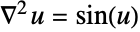
sol = NDSolve[{Subsuperscript[∇, {x}, 2]u[x] == Sin[u[x]], DirichletCondition[u[x] == 5., x == 0], DirichletCondition[u[x] == 5.1, x == π / 2]}, u, {x}∈Line[{{0}, {π / 2}}]]Plot[Evaluate[u[x] /. First[sol]], {x, 0, π / 2}]遅延型微分方程式 (2)

sol = NDSolve[{x'[t] == x[t](x[t - Pi] - x'[t - 1]), x[t /; t ≤ 0] == Cos[t]}, x, {t, 0, 8}]
Plot[Evaluate[{x[t], x'[t]} /. First[sol]], {t, 0, 8}, PlotRange -> All]Manipulate[
Module[{sol, y, t},
sol = First[y /. NDSolve[{y'[t] == λ y[t] + μ y[t - 1], y[t /; t ≤ 0] == 1 - t}, y,
{t, 0, 10}]];
If[pp, ParametricPlot[{sol[t], sol[t - 1]}, {t, 1, 10}, PlotRange -> {{-3, 3}, {-3, 3}}],
Plot[sol[t], {t, 0, 10}, PlotRange -> {{0, 10}, {-3, 3}}]]], {{pp, False, "Plot in phase plane"}, {True, False}}, {{λ, -1}, -5, 5}, {{μ, 1}, -5, 5}, FrameLabel -> ToString[y'[t] == λ y[t] + μ y[t - 1], TraditionalForm]]ハイブリッド方程式と不連続方程式 (4)
sol = NDSolve[{y'[t] == -Sign[y[t]], y[0] == 1}, y, {t, 0, 2}];Plot[y[t] /. sol, {t, 0, 2}, PlotRange -> All]sol = NDSolve[{y'[t] == a[t], y[0] == 0, a[0] == 1, WhenEvent[Mod[t, 1] == 0, a[t] -> -a[t]]}, y, {t, 0, 5}, DiscreteVariables -> a[t]];Plot[y[t] /. sol, {t, 0, 5}]

de = {x'[t] == y[t], y'[t] == -x[t] + .2 y[t] + 1};
ic = {x[0] == .5, y[0] == .5};sol = NDSolve[{de, ic, WhenEvent[And[y[t] == 0, x[t] < 0], x[t] -> -x[t]]}, {x, y}, {t, 0, 1000}];ParametricPlot[{x[t], y[t]} /. sol, {t, 0, 200}, PlotPoints -> 200]Manipulate[Module[{x0, y0, sol},
{x0, y0} = p; sol = First[NDSolve[{x'[t] == y[t], y'[t] == If[y[t] - 1 > 0, -1, .1 y[t] - x[t]], x[0] == x0, y[0] == y0}, {x, y}, {t, 0, 20}]];
ParametricPlot[{x[t], y[t]} /. sol, {t, 0, 20}, PlotRange -> {{-1.5, 1.5}, {-1.5, 1.5}}]],
{{p, {-1.5, 1.5}}, Locator}]微分代数方程式 (4)
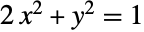
s = NDSolve[{x'[t] == y[t] ^ 2 + x[t]y[t], 2x[t] ^ 2 + y[t] ^ 2 == 1, x[0] == 0}, {x, y}, {t, 0, 10}]ParametricPlot[Evaluate[{x[t], y[t]} /. s], {t, 0, 10}, PlotRange -> All, AspectRatio -> 1]eqn = {x[t] - x'[t] + 1, x'[t] * y[t] + 2};
NDSolve[{eqn == {0, 0}, y[0] == -2}, {x, y}, {t, 0, 1}]

Det[D[eqn, {{x'[t], y'[t]}}]]eqn = {x[t] - x'[t] + 1, (x[t] + 1) * y[t] + 2};
NDSolve[{eqn == {0, 0}, y[0] == -2}, {x, y}, {t, 0, 1}]m = {{1, 0, 0}, {0, 1, 100}, {1, 1, 100}};
s = {{0, 1, 0}, {1, 1, 0}, {0, 0, 0}};
f = {Sin[t], Cos[t], 3};Length[SingularValueList[m]]r = NDSolve[{m.X'[t] == s.X[t] + f, X[0] == {0.8, 0.6, 1}}, {X}, {t, 0, 50}, Method -> {"EquationSimplification" -> "Residual"}]ParametricPlot3D[Evaluate[X[t] /. r], {t, 0, 50}, BoxRatios -> 1]微分代数方程式を指数0の系に変換し,不変量を持つ方程式として解く:
s = NDSolve[{x'[t] + y[t] == Cos[t], y'[t] + z[t] == Sin[t], x[t] == Cos[t]}, {x, y, z}, {t, 0, 5}, Method -> {"IndexReduction" -> {Automatic, "IndexGoal" -> 0}}];Plot[Evaluate[{x[t], y[t], z[t]} /. s], {t, 0, 5}, ImageSize -> 150, PlotLegends -> {x, y, z}]一般化と拡張 (1)
eqns = {Table[Derivative[1][y[i]][x] == y[i - 1][x] - y[i][x], {i, 2, 4}], {Derivative[1][y[1]][x] == -y[1][x], Derivative[1][y[5]][x] == y[4][x], y[1][0] == 1}, Table[y[i][0] == 0, {i, 2, 5}]}NDSolve[eqns, Table[y[i], {i, 5}], {x, 10}]Plot[Evaluate[Table[y[i][x], {i, 5}] /. %], {x, 0, 10}]オプション (31)
AccuracyGoalとPrecisionGoal (1)
デフォルトを使って初期条件に鋭敏に依存する天体力学方程式を解く:
eqn = z''[t] == -z[t] / (z[t]^2 + ((1 + Sin[2 π t] / 2) / 2)^2)^3 / 2;Plot[Evaluate[z[t] /. NDSolve[{eqn, z[0] == 1, z'[0] == 0}, z, {t, 0, 40}]], {t, 0, 40}]Plot[Evaluate[z[t] /. NDSolve[{eqn, z[0] == 1, z'[0] == 0}, z, {t, 0, 40}, AccuracyGoal -> 10, PrecisionGoal -> 10]], {t, 0, 40}]Plot[Evaluate[z[t] /. NDSolve[{eqn, z[0] == 1, z'[0] == 0}, z, {t, 0, 40}, AccuracyGoal -> 20, PrecisionGoal -> 20, WorkingPrecision -> 35]], {t, 0, 40}]
DependentVariables (1)
n = 1000;
vars = Table[Subscript[x, i][t], {i, n}];
eqns = Table[j = Mod[i, n] + 1;{Subscript[x, i]'[t] == 1 / (Subscript[x, i][t] + Subscript[x, j][t])^2, Subscript[x, i][0] == 1 / i}, {i, n}];Short[eqns, 3]すべての従属変数について解くが,x1についての解だけを保存する:
sol = NDSolve[eqns, Subscript[x, 1], {t, 0, 100}, DependentVariables -> vars]Plot[Subscript[x, 1][t] /. sol, {t, 0, 100}, PlotRange -> All]EvaluationMonitor (2)
Module[{c = 0}, NDSolve[{y'[x] == y[x]Cos[x + y[x]], y[0] == 1}, y, {x, 0, 30}, EvaluationMonitor :> c++];c]連続する評価の間の距離.負の距離は拒絶されたステップを表す:
ListLinePlot[Differences[Reap[NDSolve[{y'[x] == y[x]Cos[x + y[x]], y[0] == 1}, y, {x, 0, 30}, EvaluationMonitor :> Sow[x]]][[2, 1]]]]InitialSeedings (2)
NDSolveValue[{-2 u[x] Derivative[1][u][x] - Derivative[2][u][x] == 1, DirichletCondition[u[x] == 0, x == 0], DirichletCondition[u[x] == 0, x == 1]}, u, {x}∈Line[{{0}, {1}}], InitialSeeding -> {u[x] == 0}]NDSolveValue[{-2 u[x] Derivative[1][u][x] - Derivative[2][u][x] == 0, DirichletCondition[u[x] == 0, x == 0], DirichletCondition[u[x] == 1, x == 1]}, u, {x}∈Line[{{0}, {1}}], InitialSeeding -> {u[x] == x}]InterpolationOrder (1)
InterpolationOrder->Allを使ってメソッドと同じ次数の補間を得る:
Timing[a = NDSolve[{x'[t] == y[t], y'[t] == -x[t], x[0] == 1, y[0] == 0}, {x, y}, {t, 0, 1000}, InterpolationOrder -> All]]これはデフォルトで使われている補間次数よりもはるかに時間がかかる:
Timing[d = NDSolve[{x'[t] == y[t], y'[t] == -x[t], x[0] == 1, y[0] == 0}, {x, y}, {t, 0, 1000}]]Plot[Evaluate[{First[x[t] /. a], First[x[t] /. d]} - Cos[t]], {t, 0, 10}, PlotRange -> All, PlotStyle -> {Directive[Thick, Blue], Red}]MaxStepFraction (1)
積分区間の相対的に小さいサイズの特徴は見逃されることがある:
Table[Plot[Evaluate[y[x] /. NDSolve[{y''[x] + y[x] == Exp[-(1000 (x / L - 1 / 3)) ^ 2], y[0] == y'[0] == 0}, y, {x, L}]], {x, L / 4, L / 2}, PlotRange -> All], {L, {1, 10, 100, 1000}}]MaxStepFractionを使って区間の大きさにかかわらず特徴が見逃されないようにする:
Table[Plot[Evaluate[y[x] /. NDSolve[{y''[x] + y[x] == Exp[-(1000 (x / L - 1 / 3)) ^ 2], y[0] == y'[0] == 0}, y, {x, L}, MaxStepFraction -> 0.001]], {x, L / 4, L / 2}, PlotRange -> All], {L, {1, 10, 100, 1000}}]MaxSteps (1)
NDSolve[{y''[x] + x y[x] == 0, y[0] == 1, y'[0] == 0}, y, {x, 0, 200}, MaxSteps -> 10 ^ 4]
sol = NDSolve[{y''[x] + x y[x] == 0, y[0] == 1, y'[0] == 0}, y, {x, 0, 200}, MaxSteps -> 10 ^ 6]ParametricPlot[Evaluate[{y[x], y'[x]} /. First[sol]], {x, 0, 200}, ColorFunction -> Function[Hue[#3]], AspectRatio -> 1]NDSolve[{x''[t] + x[t] == 0, x[0] == 1, x'[0] == 0}, x, {t, Infinity}]
NDSolve[{x''[t] + x[t] == 0, x[0] == 1, x'[0] == 0}, x, {t, Infinity}, MaxSteps -> 20000]
MaxStepSize (2)
デフォルトのステップ制御では突然変化する特徴を見逃すことがある:
Plot[Evaluate[(y[x] /. NDSolve[{y''[x] + (1 + Sech[1000 (x - Pi)]) y[x] == 0, y[0] == 1, y'[0] == 0}, y, {x, 0, 10}]) - Cos[x]], {x, 0, 10}]MaxStepSizeの設定値を小さくしてNDSolveが特徴を確実に捉えるようにする:
Plot[Evaluate[(y[x] /. NDSolve[{y''[x] + (1 + Sech[1000 (x - Pi)]) y[x] == 0, y[0] == 1, y'[0] == 0}, y, {x, 0, 10}, MaxStepSize -> 0.01]) - Cos[x]], {x, 0, 10}] より小さい正の整数の数を計算しようとするといくつかの事象を見逃してしまう:
Block[{n = 0}, NDSolve[{y'[t] == y[t], y[-1] == E^-1, WhenEvent[Sin[π y[t]] == 0, n++]}, y, {t, 5}];n]MaxStepSizeを十分小さくして事象を一つも見逃さないようにする:
Block[{n = 0}, NDSolve[{y'[t] == y[t], y[-1] == E^-1, WhenEvent[Sin[π y[t]] == 0, n++]}, y, {t, 5}, MaxStepSize -> 0.001];n]Method (14)
TimeIntegration (5)
微分方程式の時間積分に陽的ルンゲ・クッタ法を使うように指定する:
NDSolve[{y'[x] == y[x]Cos[x + y[x]], y[0] == 1}, y, {x, 0, 30}, Method -> {"TimeIntegration" -> "ExplicitRungeKutta"}]NDSolve[{y'[x] == y[x]Cos[x + y[x]], y[0] == 1}, y, {x, 0, 30}, Method -> {"TimeIntegration" -> {"ExplicitRungeKutta", "DifferenceOrder" -> 8}}]NDSolve[{y''[t] == -y[t], y[0] == 1, y'[0] == 0}, y, {t, 0, 1}, Method -> {"TimeIntegration" -> "ExplicitEuler"}]デフォルトの解法で,連続するステップにおける x の値の違いを示す:
ListLinePlot[Differences[Reap[NDSolve[{y'[x] == y[x]Cos[x + y[x]], y[0] == 1}, y, {x, 0, 30}, StepMonitor :> Sow[x]]][[2, 1]]], DataRange -> {0, 30}]明示的なRunge–Kutta法を使うと刻み幅はあまり頻繁には変わらない:
ListLinePlot[Differences[Reap[NDSolve[{y'[x] == y[x]Cos[x + y[x]], y[0] == 1}, y, {x, 0, 30}, StepMonitor :> Sow[x], Method -> {"TimeIntegration" -> "ExplicitRungeKutta"}]][[2, 1]]], DataRange -> {0, 30}]ListLinePlot[Differences[Reap[NDSolve[{y'[x] == y[x]Cos[x + y[x]], y[0] == 1}, y, {x, 0, 30}, StepMonitor :> Sow[x], Method -> {"TimeIntegration" -> "Extrapolation"}]][[2, 1]]]]PDEDiscretization (3)
Burgersの方程式の解は急勾配になり,数値的に不安定になる可能性がある:
s1 = NDSolve[{Subscript[∂, t]u[t, x] == (1/1000)Subscript[∂, x, x]u[t, x] - u[t, x]Subscript[∂, x]u[t, x], u[0, x] == Sin[2 π x], u[t, 0] == u[t, 1]}, u, {t, 0, 2}, {x, 0, 1}]

end = Part[u   /. s1, 1, 1, 1, -1];
Plot[u[end, x] /. s1, {x, 0, 1}]s2 = NDSolve[{Subscript[∂, t]u[t, x] == (1/1000)Subscript[∂, x, x]u[t, x] - u[t, x]Subscript[∂, x]u[t, x], u[0, x] == Sin[2 π x], u[t, 0] == u[t, 1]}, u, {t, 0, 2}, {x, 0, 1}, Method -> {"PDEDiscretization" -> {"MethodOfLines", "SpatialDiscretization" -> {"TensorProductGrid", "MinPoints" -> 1000}}}]end = Part[u /. s2, 1, 1, 1, -1];
Plot[u[end, x] /. s2, {x, 0, 1}]X = Part[u /. s2, 1, 3, 2];
Plot[Max[u[t, X] /. s2], {t, 0, 2}]s2 = NDSolve[{Subscript[∂, t]u[t, x] == (1/1000)Subscript[∂, x, x]u[t, x], u[0, x] == Sin[2 π x], DirichletCondition[u[t, x] == 0, True]}, u, {t, 0, 2}, {x, 0, 1}, Method -> {"PDEDiscretization" -> {"MethodOfLines", "SpatialDiscretization" -> {"FiniteElement"}}}]時間依存シュレディンガー(Schrödinger)方程式を細分化メッシュ上で解く:
solution = NDSolve[{Inactive[Div][{{-(1/2)}} . Inactive[Grad][u[t, x], {x}], {x}] == I u^(1, 0)[t, x], u[0, x] == E^(-3I x - (1/20) x^2), DirichletCondition[u[t, x] == 0, True]}, u, {t, 0, 5}, {x, -10, 10}, Method -> {"PDEDiscretization" -> {"MethodOfLines", "SpatialDiscretization" -> {"FiniteElement", "MeshOptions" -> {"MaxCellMeasure" -> 0.1}}}}]Plot3D[Evaluate[Abs[u[t, x]] /. solution], {x, -10, 10}, {t, 0, 5}, PlotPoints -> 50, AxesLabel -> {x, t}]BoundaryValues (1)
sol0 = First[NDSolve[{x''[t] + Sin[x[t]] == 0, x[0] == x[10] == 0}, x, t]]デフォルトオプションを使うと,このメソッドでは自明な解が求まる:
Table[x[t] /. sol0, {t, 0, 10}]"Shooting"メソッドでデフォルトとは異なる初期条件を指定して別の解を求める:
sols = Map[First[NDSolve[{x''[t] + Sin[x[t]] == 0, x[0] == x[10] == 0}, x, t, Method -> "BoundaryValues" -> {"Shooting", "StartingInitialConditions" -> {x[0] == 0, x'[0] == #}}]]&,
	{1.5, 1.75, 2}];
Plot[Evaluate[x[t] /. sols], {t, 0, 10}, PlotStyle -> {Brown, Blue, Green}]
DiscontinuityProcessing (1)
NDSolveはSignのような不連続関数の処理を自動的に行う:
sol1 = NDSolve[{x'[t] == Sign[1 - x[t]], x[0] == 0}, x, {t, 0, 2}]この処理が使用できなくなっていると,NDSolveは不連続点で止まる可能性がある:
NDSolve[{x'[t] == Sign[1 - x[t]], x[0] == 0}, x, {t, 0, 2}, Method -> {"DiscontinuityProcessing" -> False}]
使う時間積分法によっては,解が非常に不正確になる場合もある:
sol2 = NDSolve[{x'[t] == Sign[1 - x[t]], x[0] == 0}, x, {t, 0, 2}, Method -> {"DiscontinuityProcessing" -> False, "TimeIntegration" -> "Extrapolation"}]Plot[{x[t] /. sol1 , x[t] /. sol2}, {t, 0, 2}]解を求める同等の方法として"DiscontinuitySignature"の使用が考えられる:
sol3 = NDSolve[{Derivative[1][x][t] == v[t], WhenEvent[1 == x[t], v[t] -> "DiscontinuitySignature"], x[0] == 0, v[0] == 1}, {x, v}, {t, 0, 2}, DiscreteVariables -> {Element[v, {-1, 0, 1}]}]Table[(x[t] /. sol1) - (x[t] /. sol3), {t, 0, 2, .25}]Plot[v[t] /. sol3, {t, 0, 2}]EquationSimplification (2)
NDSolve[{Derivative[1][x][t] ^ 2 + x[t] ^ 2 == 1, x[0] == 1 / 2}, x, {t, 0, 10 Pi}]

剰余を形成し,微分代数方程式系として解くことで1つの解を求めることができる:
s1 = NDSolve[{Derivative[1][x][t] ^ 2 + x[t] ^ 2 == 1, x[0] == 1 / 2}, x, {t, 0, 10 Pi}, Method -> {"EquationSimplification" -> "Residual"}]他の解の分枝は  の一定の値を指定することで得ることができる:
s2 = NDSolve[{Derivative[1][x][t] ^ 2 + x[t] ^ 2 == 1, x[0] == 1 / 2, x'[0] == -Sqrt[3 / 4]}, x, {t, 0, 10 Pi}, Method -> {"EquationSimplification" -> "Residual"}]Plot[Evaluate[x[t] /. {s1, s2}], {t, 0, 10 Pi}]サブオプション"SimplifySystem"->Trueを使うと,NDSolveは十分に単純な形の成分については記号解を使う:
sol = NDSolve[{x'[t] + y[t] == Sin[t], y'[t] + z[t] == Sin[t], y[t] == Cos[t], x[0] == 1}, {x, y, z}, {t, 0, 2Pi}, Method -> {"EquationSimplification" -> {Automatic,
"SimplifySystem" -> True}}]Plot[Evaluate[{x[t], y[t], z[t]} /. sol], {t, 0, 2Pi},
PlotLegends -> {x[t], y[t], z[t]}]IndexReduction (1)
eqns = {x''[t] == T[t]x[t], y''[t] == T[t] y[t] - 1, x[t] ^ 2 + y[t] ^ 2 == 1};
init = {x[0] == 1, y[0] == 0, y'[0] == -14 / 10};
vars = {x, y, T};NDSolve[{eqns, init}, vars, {t, 0, 10}]
s1 = First[NDSolve[{eqns, init}, vars, {t, 0, 10}, Method -> {"IndexReduction" -> True}]]s2 = First[NDSolve[{eqns, init}, vars, {t, 0, 10}, Method -> {"IndexReduction" -> {True, "ConstraintMethod" -> "Projection"}}]]時間ステップの2つの解についての暗黙のエネルギー制約をプロットする:
energy[sol_] := Module[{times = Part[x /. sol, 3, 1], es},
es[t_] = 1 + y[t] + (1/2) (-y[t] Derivative[1][x][t] + x[t] Derivative[1][y][t])^2 /. sol;Transpose[{times, es[times] - es[0]}]];ListPlot[{energy[s1], energy[s2]}]DAEInitialization (1)
初期化の前進コロケーションを使って0におけるAbsにまつわる問題を避ける:
NDSolve[{x'[t] == Abs[u[t]], u[t] == Sin[t], y[t] == x[t], y[0] == 10}, {x, y, u}, {t, 0, 10}, Method -> {"DAEInitialization" -> {"Collocation", "CollocationDirection" -> "Forward"}}]NormFunction (1)
さまざまな誤差推定のノルムを使った実際の解の誤差をプロットする:
L = 10;Table[sol[p] = NDSolve[{D[u[t, x], t, t] == D[u[t, x], x, x], u[0, x] == Exp[-x ^ 2], Derivative[1, 0][u][0, x] == -Exp[-x ^ 2], u[t, -L] == u[t, L]}, u, {t, 0, 4 L}, {x, -L, L}, NormFunction -> (Norm[#, p]&), Method -> {"MethodOfLines", "SpatialDiscretization" -> {"TensorProductGrid", "MaxPoints" -> 125, "MinPoints" -> 125, "DifferenceOrder" -> "Pseudospectral"}}];
Plot[Evaluate[(u[4L, x] /. sol[p])  -   (Exp[-x ^ 2] - 2Sqrt[π])], {x, -L, L}, PlotRange -> All], {p, {1, 2, 3, ∞}}]


Plot3D[u[t, x] /. sol[1], {t, 0, 40}, {x, -L, L}, Mesh -> False, PlotPoints -> 20]
StartingStepSize (1)
区間が非常に大きい場合には,始点近くの長続きしない特徴は見逃されることがある:
feature[t_ ? NumberQ] := If[t < 1, t Sin[10 Pi t], 0];sol = NDSolve[{x''[t] + 10 ^ -4 x[t] == feature[t], x[0] == x'[0] == 0}, x, {t, 0, 10000}]Max[Abs[x[RandomReal[{0, 10000}, 10000]] /. sol]]sol = NDSolve[{x''[t] + 10 ^ -4 x[t] == feature[t], x[0] == x'[0] == 0}, x, {t, 0, 10000}, StartingStepSize -> 0.1]{Plot[x[t] /. sol, {t, 0, 2}], Plot[x[t] /. sol, {t, 0, 10000}]}StepMonitor (3)
解の処理の中でステップが取られる各点における解をプロットする:
ListLinePlot[Reap[NDSolve[{y'[x] == y[x]Cos[x + y[x]], y[0] == 1}, y, {x, 0, 30}, StepMonitor :> Sow[{x, y[x]}]]][[2, 1]]]Module[{c = 0}, NDSolve[{y'[x] == y[x]Cos[x + y[x]], y[0] == 1}, y, {x, 0, 30}, StepMonitor :> c++];c]ListLinePlot[Differences[Reap[NDSolve[{y'[x] == y[x]Cos[x + y[x]], y[0] == 1}, y, {x, 0, 30}, StepMonitor :> Sow[x]]][[2, 1]]]]WorkingPrecision (1)
T = 200 Pi;
Timing[y[T] /. NDSolve[{y''[x] + y[x] == 0, y[0] == 0, y'[0] == 1}, y, {x, 0, T}, MaxSteps -> Infinity]]Timing[y[T] /. NDSolve[{y''[x] + y[x] == 0, y[0] == 0, y'[0] == 1}, y, {x, 0, T}, WorkingPrecision -> 32, MaxSteps -> 10 ^ 6]]作業精度を高くすると,"Extrapolation"メソッドが非常に効果的になることもある:
Timing[y[T] /. NDSolve[{y''[x] + y[x] == 0, y[0] == 0, y'[0] == 1}, y, {x, 0, T}, WorkingPrecision -> 32, Method -> "Extrapolation"]]T = 200 Pi;
Timing[y[T] /. NDSolve[{y''[x] + y[x] == 0, y[0] == 0, y'[0] == 1}, y, {x, 0, T}]]Timing[y[T] /. NDSolve[{y''[x] + y[x] == 0, y[0] == 0, y'[0] == 1}, y, {x, 0, T}, WorkingPrecision -> 32, MaxSteps -> Infinity]]作業精度を高くすると,"Extrapolation"メソッドが非常に効果的になることもある:
Timing[y[T] /. NDSolve[{y''[x] + y[x] == 0, y[0] == 0, y'[0] == 1}, y, {x, 0, T}, WorkingPrecision -> 32, Method -> "Extrapolation"]]アプリケーション (42)
常微分方程式 (5)
二重ポテンシャル井戸中の粒子についてのDuffingの方程式のシミュレーションを行う:
s = NDSolve[{x''[t] + 0.15x'[t] - x[t] + x[t] ^ 3 == 0.3Cos[t], x[0] == -1, x'[0] == 1}, x, {t, 0, 50}]Plot[Evaluate[x[t] /. s], {t, 0, 50}]s = NDSolve[{x''[t] + 0.15x'[t] - x[t] + x[t] ^ 3 == 0.3Cos[t],
x[0] == -1, x'[0] == 1.001}, x, {t, 0, 50}]Plot[Evaluate[x[t] /. s], {t, 0, 50}]ローレンツ(Lorenz)方程式 [詳細]:
s = NDSolve[{Derivative[1][x][t] == -3 (x[t] - y[t]), Derivative[1][y][t] == -x[t] z[t] + 26.5 x[t] - y[t], Derivative[1][z][t] == x[t] y[t] - z[t], x[0] == z[0] == 0, y[0] == 1}, {x, y, z}, {t, 0, 200}]ParametricPlot3D[Evaluate[{x[t], y[t], z[t]} /. s], {t, 0, 200}, PlotPoints -> 1000, ColorFunction -> (Hue[#4]&)]ロトカ・ヴォルテラの捕食者と被食者の方程式 [詳細]:
NDSolve[{y'[t] == y[t](x[t] - 1), x'[t] == x[t](2 - y[t]), x[0] == 1, y[0] == 2.7}, {x, y}, {t, 0, 10}]ParametricPlot[Evaluate[{x[t], y[t]} /. First[%]], {t, 0, 10}]Gavrilov・Shilnikovモデルで「blue sky catastrophe」軌道の外観を見る:
eqns = {
	x'[t] == x[t](2 + μ - 10(x[t] ^ 2 + y[t] ^ 2)) + z[t] ^ 2 + y[t] ^ 2 + 2 y[t],
	y'[t] == -z[t] ^ 3 - (1 + y[t])(z[t] ^ 2 + y[t] ^ 2 + 2 y[t]) - 4 x[t] + μ y[t],
z'[t] == (1 + y[t]) z[t] ^ 2 + x[t] ^ 2 - ϵ};Table[Block[{ϵ = 0.0357, T = 1000},
sol = First[NDSolve[{eqns, x[0] == y[0] == z[0] == 1}, {x, y, z}, {t, 0, T}]];
ParametricPlot3D[Evaluate[{x[t], y[t], z[t]} /. sol], {t, T / 4, T}, BoxRatios -> 1, PlotPoints -> 1000, PlotRange -> All]], {μ, .455, .456, .001}]簡約された3体(3-body)問題 [詳細]:
eqn = z''[t] == -(z[t]/(z[t]^2 + ((1/2) (1 + 0.1 Sin[2 Pi t]))^2)^3 / 2);NDSolve[{eqn, z[0] == 1, z'[0] == 0}, z, {t, 0, 30}]Plot[Evaluate[z[t] /. %], {t, 0, 30}]eqn = D[z[t, s], t, t] == -(z[t, s]/(z[t, s]^2 + ((1/2) (1 + 0.1 Sin[2 Pi t]))^2)^3 / 2);sol = NDSolve[{eqn, z[0, s] == s, Derivative[1, 0][z][0, s] == 0}, z, {t, 0, 10}, {s, 1, 2}]Plot3D[Evaluate[z[tp, z0] /. sol], {tp, 0, 10}, {z0, 1, 2}]偏微分方程式 (17)
PDEModelsの概要には,さまざまな分野からの詳細な説明付きのPDEモデルの大規模コレクションが収められている.
表面を周期的に暖めた場合の深さ x における地熱の簡単なモデル:
NDSolve[{D[u[t, x], t] == D[u[t, x], x, x], u[0, x] == 0, u[t, 0] == Sin[t], u[t, 5] == 0}, u, {t, 0, 10}, {x, 0, 5}]Plot3D[Evaluate[u[t, x] /. %], {t, 0, 10}, {x, 0, 5}, PlotRange -> All]s = NDSolve[{Subscript[∂, t, t]u[t, x] == Subscript[∂, x, x]u[t, x], u[0, x] == E^-x^2, u^(1, 0)[0, x] == 0, u[t, -10] == u[t, 10]}, u, {t, 0, 40}, {x, -10, 10}]DensityPlot[Evaluate[First[u[t, x] /. s]], {t, 0, 40}, {x, -10, 10}, PlotPoints -> 30]Wolframの非線形波動方程式 [詳細]:
s = NDSolve[{Subscript[∂, t, t]u[t, x] == Subscript[∂, x, x]u[t, x] + (1 - u[t, x]^2) (1 + 2 u[t, x]), u[0, x] == E^-x^2, u^(1, 0)[0, x] == 0, u[t, -10] == u[t, 10]}, u, {t, 0, 10}, {x, -10, 10}]Plot3D[Evaluate[u[t, x] /. s], {t, 0, 10}, {x, -10, 10}]DensityPlot[Evaluate[u[-t, x] /. s], {x, -10, 10}, {t, 0, -10}]Wolframのディリクレ条件がある非線形波動方程式[詳細]を使ってモデル化する.
ics = {u[0, x] == Exp[-x ^ 2], Derivative[1, 0][u][0, x] == 0};bcs = DirichletCondition[u[t, x] == 0, True];sol = NDSolve[{(1 + 2 u[t, x]) (-1 + u[t, x]^2) + Inactive[Div][-Inactive[Grad][u[t, x], {x}], {x}] + u^(2, 0)[t, x] == 0, ics, bcs}, u, {t, 0, 10}, {x, -10, 10}]Plot3D[u[t, x] /. sol, {x, -10, 10}, {t, 0, 10}, ...]NDSolve[{D[u[t, x, y], t, t] == D[u[t, x, y], x, x] + D[u[t, x, y], y, y] / 2 + (1 - u[t, x, y] ^ 2)(1 + 2u[t, x, y]), u[0, x, y] == E^-(x^2 + y^2), u[t, -5, y] == u[t, 5, y], u[t, x, -5] == u[t, x, 5], u^(1, 0, 0)[0, x, y] == 0}, u, {t, 0, 4}, {x, -5, 5}, {y, -5, 5}]Table[Plot3D[Evaluate[u[t, x, y] /. %], {x, -5, 5}, {y, -5, 5}, PlotRange -> All], {t, 1, 4}]非線形シュレディンガー(Schrödinger)方程式における周期的なソース項によって駆動される移動ソリトン:
L = 50;
sol = NDSolve[{I D[u[t, x], t] + D[u[t, x], x, x] + 2 Abs[u[t, x]] ^ 2 u[t, x] == 0.1 (1 - Cos[Pi x / L]), u[0, x] == Sech[x] Exp[I x], u[t, -L] == u[t, L]}, u, {t, 0, 10}, {x, -L, L}]Plot3D[Evaluate[Abs[u[t, x] /. First[sol]]], {t, 0, 10}, {x, -L, L}, PlotPoints -> 60, MaxRecursion -> 3, Mesh -> None]非線形シュレディンガー方程式の周期ポテンシャルのもとで移動するソリトン:
L = 20;
sol = NDSolve[{I D[u[t, x], t] + D[u[t, x], x, x] + 2 Abs[u[t, x]] ^ 2 u[t, x] + 0.1 (1 - Cos[Pi x / L]) u[t, x] == 0, u[0, x] == Sech[x]Exp[I x], u[t, -L] == u[t, L]}, u, {t, 0, 15}, {x, -L, L}]Plot3D[Abs[u[t, x] /. First[sol]], {t, 0, 15}, {x, -L, L}, PlotPoints -> 60, PlotRange -> All, MaxRecursion -> 3]Korteweg-de Vries (KdV)方程式を標準形で定義する:
KdV = {D[u[x, t], t] + D[u[x, t], {x, 3}] + 6u[x, t]D[u[x, t], x] == 0}sol = NDSolve[{KdV, u[x, 0] == 2 - 2 Tanh[(1/4) + x]^2, u[-50, t] == u[50, t]}, u, {x, -50, 50}, {t, 0, 10}]Plot[Evaluate[Table[u[x, t] /. First[sol], {t, 1, 12, 3}]], {x, -5, 50}, PlotRange -> All, Filling -> Axis, Epilog -> {Arrow[{{5, 1.6}, {9, 1.6}}], Arrow[{{17, 1.6}, {21, 1.6}}], Arrow[{{29, 1.6}, {33, 1.6}}], Arrow[{{41, 1.6}, {45, 1.6}}]}]KdV = {D[u[x, t], t] + D[u[x, t], {x, 3}] - 6u[x, t]D[u[x, t], x] == 0}sol = NDSolve[{KdV, u[x, 0] == -6 Sech[x]^2, u[-50, t] == u[50, t]}, u, {x, -50, 50}, {t, 0, 10}, Method -> {"MethodOfLines", "SpatialDiscretization" -> {"TensorProductGrid", "MaxPoints" -> 5000, "MinPoints" -> 5000}, Method -> "StiffnessSwitching"}]ListAnimate[Plot[#, {x, -50, 50}, PlotRange -> All]& /@ Table[u[x, t] /. First[sol], {t, 0, 10, 0.1}], SaveDefinitions -> True]Ω = RegionUnion[Rectangle[{0, 0}, {1, 1 / 2}], Rectangle[{1, 1 / 10}, {2, 2 / 5}]];
{xVel, yVel} = {u, v} /. First[NDSolve[{{Inactive[Div][{{-μ, 0}, {0, -μ}} . Inactive[Grad][u[x, y], {x, y}], {x, y}] + p^(1, 0)[x, y], Inactive[Div][{{-μ, 0}, {0, -μ}} . Inactive[Grad][v[x, y], {x, y}], {x, y}] + p^(0, 1)[x, y], u^(1, 0)[x, y] + v^(0, 1)[x, y]} == {0, 0, 0} /. μ -> 1, {
DirichletCondition[u[x, y] == 4 * 0.3 * y * (0.5 - y) / (0.41) ^ 2, x == 0.], DirichletCondition[{u[x, y] == 0., v[x, y] == 0.}, 0 < x < 2],
DirichletCondition[p[x, y] == 0., x == 2]}}, {u, v, p}, {x, y}∈Ω, Method -> {"FiniteElement", "InterpolationOrder" -> {u -> 2, v -> 2, p -> 1}, "MeshOptions" -> {"MaxCellMeasure" -> 0.0005}}]];VectorPlot[{xVel[x, y], yVel[x, y]}, {x, y}∈Ω, AspectRatio -> Automatic, StreamPoints -> 6, StreamColorFunctionScaling -> False]vars = {Θ[x], {x}};
pars = <|"ThermalConductivity" -> 0.026, "HeatSource" -> 1|>;
Ω = Line[{{0}, {1}}];
eqn = HeatTransferPDEComponent[vars, pars] == 0Tfun = NDSolve[{eqn, HeatTemperatureCondition[x == 0, vars, pars, <|"SurfaceTemperature" -> 0|>]}, Θ, x∈Ω]Plot[Θ[x] /. Tfun, {x}∈Ω]過度音圧場についてのモデル変数 vars をモデルパラメータ pars で定義する:
vars = {p[t, x], t, {x}};
pars = <|"SoundSpeed" -> 343, "MassDensity" -> 1.2|>;
p0 = D[0.125 Erf[(x - 0.5) / 0.15], x];
ics = {p[0, x] == p0, Derivative[1, 0][p][0, x] == -343 * D[p0, x]};eqn = AcousticPDEComponent[vars, pars] == AcousticSoundHardValue[x == 1, vars, pars]pfun = NDSolve[{eqn, ics}, p, {t, 0, 0.003}, x∈Line[{{0}, {1}}]]Manipulate[Plot[Evaluate[p[t, x] /. pfun], {x, 0, 1}, ...], {{t, 0}, 0, 0.003, 10 ^ -4}, Rule[...]]1つの反応速度でさまざまな材料を通過する1D化学種の移動をモデル化する.右辺と左辺はそれぞれ質量濃度と流入条件に従う:

vars = {c[x], {x}};
Ω = Line[{{0}, {1}}];領域  でアクティブな,物質移動モデルパラメータ種拡散率
 と反応率
 を指定する:
pars = <|"DiffusionCoefficient" -> 0.01, "MassReactionRate" -> If[x > 1 / 2, 1, 0]|>;Subscript[Γ, flux] = MassFluxValue[x == 0, vars, pars, <|"MassFlux" -> 1|>]Subscript[Γ, C] = MassConcentrationCondition[x == 1, vars, pars, <|"MassConcentration" -> 0|>]eqn = MassTransportPDEComponent[vars, pars] == Subscript[Γ, flux]cfun = NDSolve[{eqn, Subscript[Γ, C]}, c, x∈Ω]Show[Plot[Evaluate[c[x] /. cfun], x∈Ω, Rule[...]], Graphics[...]]eqn = {u[t, x, y] (f + v[t, x, y]^2) + Inactive[Div][(-c1)*Inactive[Grad][u[t, x, y], {x, y}], {x, y}] + u^(1, 0, 0)[t, x, y] == f, v[t, x, y] (f + k - u[t, x, y] v[t, x, y]) + Inactive[Div][(-c2)*Inactive[Grad][v[t, x, y], {x, y}], {x, y}] + v^(1, 0, 0)[t, x, y] == 0} //. {c1 -> 2 * 10 ^ -5, c2 -> c1 / 4, f -> 1 / 25, k -> 3 / 50};初期条件として, なら
 および
 でそれ以外の場合は0と設定する:
ics = {u[0, x, y] == 1 / 2, v[0, x, y] == If[x ^ 2 + y ^ 2 <= 1 / 40, 1, 0]};

bcs = DirichletCondition[{u[t, x, y] == 0, v[t, x, y] == 0}, True];sol = NDSolve[{eqn, bcs, ics}, {u, v}, {x, y}∈Disk[], {t, 0, 3000}, Method -> {"PDEDiscretization" -> {"MethodOfLines", "SpatialDiscretization" -> {"FiniteElement", "MeshOptions" -> {"MaxCellMeasure" -> 0.003}}}}];frames = Table[ContourPlot[v[t, x, y] /. sol, {x, -1, 1}, {y, -1, 1}, ...], {t, 100, 2000, 25}];
ListAnimate[frames, Rule[...]]eqn = {u^(1, 0)[t, x] + Inactive[Div][-Inactive[Grad][u[t, x], {x}], {x}] + Inactive[Div][-Inactive[Grad][v[t, x], {x}], {x}] - u[t, x] + (u[t, x] - 2 v[t, x]) (u[t, x]^2 + v[t, x]^2) == 0, v^(1, 0)[t, x] + Inactive[Div][Inactive[Grad][u[t, x], {x}], {x}] + Inactive[Div][-Inactive[Grad][v[t, x], {x}], {x}] - v[t, x] + (2 u[t, x] + v[t, x]) (u[t, x]^2 + v[t, x]^2) == 0};exp[x_] := If[x < Log[$MinMachineNumber], 0., Exp[x]]
ics = {u[0, x] == 1 - exp[-x ^ 2], v[0, x] == exp[-(10 - x) ^ 2]};bcs = {u[t, -50] == 1, u[t, 50] == 1, v[t, -50] == 0, v[t, 50] == 0};sol = NDSolve[{eqn, ics, bcs}, {u, v}, {t, 0, 40}, {x, -50, 50}, Method -> {"MethodOfLines", "SpatialDiscretization" -> {"FiniteElement", "MeshOptions" -> {"MaxCellMeasure" -> 0.4}}}];DensityPlot[Evaluate[Sqrt[(u[t, x] ^ 2 + v[t, x] ^ 2) /. sol]], {x, -50, 50}, {t, 0, 40}, ...]ブラックショールズ方定式.目標は,ブラック・ショールズ・モデルを使ってヨーロピアン・バニラ・コール・オプションの価格を決定することである.ここで,原資産価格  と行使価格
 はどちらも
 ドル,無リスク金利
 は
 ,資産のボラティリティ
 は
 ,オプションの満期期間
 は1年である.
pars = {tEnd -> 1, k -> 100, σ -> 0.2, r -> 0.05}
{lower, upper} = {0, 3k} /. parsBSPDE = -r V[t, s] + r s V^(0, 1)[t, s] + (1/2) s^2 σ^2 V^(0, 2)[t, s] + V^(1, 0)[t, s] == 0 /. parsterminalBC = V[tEnd, s] == Max[0, s - k] /. pars境界条件は,資産価格が非常に低い下界においてオプションの価値が0になるように選択される.上界の条件はプット・コール・パリティから来る.
bcs = {DirichletCondition[V[t, s] == upper - k E^-r(tEnd - t), s == upper], DirichletCondition[V[t, s] == 0, s == lower]} /. parssol = NDSolve[{BSPDE, terminalBC, bcs}, V, {t, 0, tEnd} /. pars, {s, lower, upper}, Method -> {"MethodOfLines", "SpatialDiscretization" -> {"FiniteElement", "MeshOptions" -> {"MaxCellMeasure" -> 0.1}}}]時点  における資産価格
 についてオプションの値をチェックする:
V[0, 100] /. sol[[1]]Plot3D[V[t, s] /. sol, {s, 50, 150}, {t, 0, 1}, ...]FinancialDerivative関数を使って関数を定義して,オプションの価格を取得する:
optionPrice[s0_] := FinancialDerivative@@ReplaceAll[{{"European", "Call"}, {"StrikePrice" -> k, "Expiration" -> tEnd}, {"InterestRate" -> r, "Volatility" -> σ, "CurrentPrice" -> s0}}, pars]FinancialDerivativeが与える慣習的に真である値を調べる:
optionPrice[100]trueVal = optionPrice[100];
numericalVal = V[0, 100] /. sol[[1]];
PercentForm[(Abs[trueVal - numericalVal]/trueVal)]時点 における数値解と慣習的に真である解の間の差をプロットする:
Plot[optionPrice[s0] - V[0, s0] /. sol, {s0, 0, 200} /. pars, ...]遅延型微分方程式 (1)
呼吸力学におけるMackey–Glassの遅延型微分方程式の解を見る:
Manipulate[
	Module[{sol, x, t},
	sol = First[ NDSolve[{x'[t] == a x[t - τ] / (1 + x[t - τ] ^ 10)  - b  x[t], x[t /; t ≤ 0] == 1 / 2}, x, {t, 0, 500}]];
	ParametricPlot[Evaluate[{x[t], x[t - τ]} /. sol], {t, 300, 500}, PlotRange -> {{0, 2}, {0, 2}}]], {{a, .2}, 0, 1}, {{b, .1}, 0, 1},
	{{τ, 17}, 1, 20}]
ハイブリッド微分方程式 (5)
それぞれのバウンドで速度の95%を保ちながらバウンドするボールのシミュレーションを行う:
NDSolve[{y''[t] == -9.81, y[0] == 5, y'[0] == 0, WhenEvent[y[t] == 0, y'[t] -> -0.95y'[t]]}, y, {t, 0, 10}];Plot[y[t] /. %, {t, 0, 10}]ballsteps = NDSolve[{x''[t] == 0, y''[t] == -9.8, y[0] == 6, y'[0] == 0, x[0] == 0, x'[0] == 1, a[0] == 5, WhenEvent[Mod[x[t], 1] == 0, If[a[t] > 0, a[t] -> a[t] - 1, "RemoveEvent"]], WhenEvent[y[t] == a[t], {x'[t], y'[t]} -> .9{x'[t], -y'[t]}]}, {x, y, a}, {t, 0, 15}, DiscreteVariables -> {a}];Show[ParametricPlot[Evaluate[{{x[t], y[t]}, {x[t], a[t]}} /. ballsteps], {t, 0, 15}], Plot[{0, Floor[6 - x]}, {x, -1, 15}, Filling -> {2 -> 0}, Exclusions -> None], Frame -> {{True, False}, {True, False}}, FrameLabel -> {"x", "y"}]線形振動解が負の  軸と交差するたびにこれを
 軸に沿って反射させる:
de[δ_] := {Subscript[x, 1]'[t] == Subscript[x, 2][t], Subscript[x, 2]'[t] == -Subscript[x, 1][t] + 2δ Subscript[x, 2][t] + 1};
ic = {Subscript[x, 1][0] == .5, Subscript[x, 2][0] == .5};{sol, {points}} = NDSolve[{de[0.1], ic, WhenEvent[And[Subscript[x, 2][t] == 0, Subscript[x, 1][t] < 0], {Subscript[x, 1][t] -> -Subscript[x, 1][t], Sow[-Subscript[x, 1][t]]}]}, {Subscript[x, 1], Subscript[x, 2]}, {t, 0, 1000}]//Reap;Map[ParametricPlot[{Subscript[x, 1][t], Subscript[x, 2][t]} /. sol, {t, 0, #}, PlotPoints -> 500, PlotRange -> {{-1, 3}, {-2, 2}}]&, {10, 100, 400}]
Grid[{{Histogram[points, {-1, 0, .05}]}, {ParametricPlot[{Subscript[x, 1][t], Subscript[x, 2][t]} /. sol, {t, 0, 1000}, PlotRange -> {{-1, 0}, {-0.3, 0}}, PlotPoints -> 2000, Axes -> None]}}]sol[ω_] := With[{r = 0.95},
NDSolve[{u'[t] == v[t], v'[t] == -u[t] + Cos[ω t], u[0] == 0, v[0] == 0, WhenEvent[u[t] == 0, v[t] -> -r v[t]]}, {u, v}, {t, 0, 300}]];Table[ParametricPlot[Evaluate[{u[t], v[t]} /. sol[ω]], {t, 200, 300}, PlotPoints -> 200, PlotRange -> {{-.1, 1}, {-1, 1}}], {ω, {3, 2.76, 2.9}}]system = {x''[t] + .1x'[t] + x[t] == 0, x[0] == 1, x'[0] == 0};
control = WhenEvent[Mod[t, 1], x'[t] -> x'[t] + 1];sol = NDSolve[{system, control}, x, {t, 0, 100}]Plot[Evaluate[{x[t], x'[t]} /. sol], {t, 0, 100}, PlotPoints -> 120]ParametricPlot[{x[t], x'[t]} /. sol, {t, 90, 100}, AspectRatio -> 1]機械系 (3)
直交座標で振子の動きをモデル化する.ニュートンの運動の第2法則  および
 を示力図とともに使って支配方程式を導く:
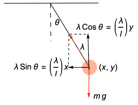
deqns = {x''[t] == λ[t] x[t], y''[t] == λ[t] y[t] - 9.81};
aeqns = {x[t]^2 + y[t]^2 == 1^2};
ics = {x[0] == 1, y'[0] == 1};sol1 = NDSolve[{deqns, aeqns, ics}, {x, y, λ}, {t, 0, 5}, Method -> {"IndexReduction" -> True}];Plot[Evaluate[{x[t], y[t]} /. sol1], {t, 0, 5}]deqns2 = {x''[t] == λ[t]x[t] - 0.5 x'[t], y''[t] == λ[t] y[t] - 9.8 - 0.5 y'[t]};sol2 = NDSolve[{deqns2, aeqns, ics}, {x, y, λ}, {t, 0, 20}, Method -> {"IndexReduction" -> True}];Plot[Evaluate[{x[t], y[t]} /. sol2], {t, 0, 20}]
aeqns3 = {Sqrt[x[t]^2 + y[t]^2](1 + λ[t] κ) == 1};
κ = 5 10 ^ -4;sol3 = Quiet@NDSolve[{deqns, aeqns3, ics}, {x, y, λ}, {t, 0, 5}, Method -> {"IndexReduction" -> True}, AccuracyGoal -> 6];Plot[Evaluate[{x[t], y[t]} /. sol3], {t, 0, 5}]水平平面から放たれる,単位質量と単位長の二重振子をモデル化する.まず,ニュートンの運動の第2法則を使って方程式を導く:
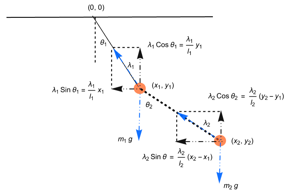
deqns = {x1''[t] == λ1[t] x1[t] - λ2[t](x2[t] - x1[t]), y1''[t] == λ1[t] y1[t] - λ2[t](y2[t] - y1[t]) - 9.81,
	x2''[t] == λ2[t](x2[t] - x1[t]), y2''[t] == λ2[t] (y2[t] - y1[t]) - 9.81};
aeqns = {x1[t]^2 + y1[t]^2 == 1, (x2[t] - x1[t])^2 + (y2[t] - y1[t])^2  == 1};
ics = {x1[0] == 1, y1'[0] == 1, x2[0] == 2, y2'[0] == 1};
方程式と制約条件を不変量として強制することで,系のシミュレーションを行う:
sol = Quiet@NDSolve[{deqns, aeqns, ics}, {x1, y1, x2, y2, λ1, λ2}, {t, 0, 15}, Method -> {"IndexReduction" -> {True, "ConstraintMethod" -> "Projection"}}] ;Animate[Graphics[{{Thickness[0.02], Red, Line[{{0, 0}, {x1[t], y1[t]}}]}, {Thickness[0.02], Blue, Line[{{x1[t], y1[t]}, {x2[t], y2[t]}}]}} /. sol, PlotRange -> {{-2.1, 2.1}, {0.6, -2.1}}, Frame -> True], {t, 0, 15}, SaveDefinitions -> True, AnimationRunning -> False]動いているコンベヤベルト上の,粘度摩擦,クーロン摩擦,ストライベック摩擦,静摩擦を含むまざまな摩擦推力  を使ったバネで壁に固定されたブロックをモデル化する.各モデルについて位置と速度を比較する:
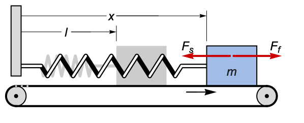
m = l = 1.;
beltv[t_] = .1;
spring[x_] = 1000.(l - x);sys := {m x''[t] == spring[x[t]] + friction[x'[t]], x[0] == 1, x'[0] == 0};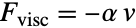
viscous[v_] := -30.(v - beltv[t]);
friction[v_] := viscous[v];{pos1, vel1} = NDSolveValue[sys, {x[t], x'[t]}, {t, 0, 2}];{Plot[{pos1}, {t, 0, 1}, PlotRange -> All], Plot[{vel1, beltv[t]}, {t, 0, 1}, PlotRange -> All]}
coulomb[v_] := -25.Sign[v - beltv[t]];
friction[v_] := viscous[v] + coulomb[v];{pos2, vel2} = NDSolveValue[sys, {x[t], x'[t]}, {t, 0, 20}];{Plot[{pos2}, {t, 0, 1}, PlotRange -> All], Plot[{vel2, beltv[t]}, {t, 0, 1}, PlotRange -> All]}
stribeck[v_] := -.3Sign[v]Exp[-2Abs[v]];
friction[v_] := viscous[v] + coulomb[v] + stribeck[v];{pos3, vel3} = NDSolveValue[sys, {x[t], x'[t]}, {t, 0, 20}];{Plot[{pos3}, {t, 0, 1}, PlotRange -> All], Plot[{vel3, beltv[t]}, {t, 0, 1}, PlotRange -> All]}ストライベック摩擦は,バネの力がベルト表面の粗さに依存する値 μ を超えるまでブロックを一定の位置に保つ.離散変量 stuck は,ブロックが動かない場合は1に,それ以外の場合は0に設定する:
friction[v_] := viscous[v] + coulomb[v] + stribeck[v];staticsys := {x''[t] == If[stuck[t] == 1, beltv'[t], spring[x[t]] + friction[x'[t]]], x[0] == 1, x'[0] == 0};バネの力が μ より小さいかどうか,またブロックがベルトと相対的に移動していないかどうかをチェックする:
μ = 100;
stick = WhenEvent[x'[t] == beltv[t], stuck[t] -> Boole[spring[x[t]]^2 < μ^2]];
slip = WhenEvent[spring[x[t]]^2 > μ^2, stuck[t] -> 0];{pos4, vel4} = NDSolveValue[{staticsys, stick, slip, stuck[0] == 0}, {x[t], x'[t]}, {t, 0, 8}, DiscreteVariables -> stuck[t]];ブロックは繰り返しベルトに着いて動かなくなり,次にバネの力によって引き戻される:
{Plot[{pos4}, {t, 0, 2}, PlotRange -> All], Plot[{vel4, beltv[t]}, {t, 0, 2}, PlotPoints -> 100, PlotRange -> All]}Plot[{pos1, pos2, pos3, pos4}, {t, 0, 2}, PlotRange -> {0.9, 1.1}, PlotLegends -> {"viscous", "Coulomb", "Stribeck", "static"}]電気系 (6)
時間  ,電圧
 に対するRLC回路のステップ応答のシミュレーションを行う:
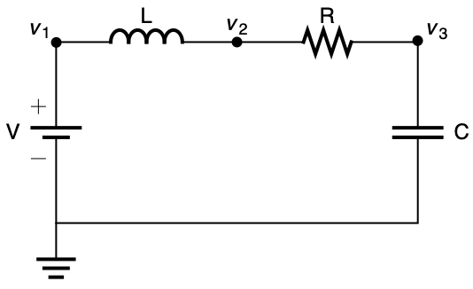
成分法則を接続に関するキルヒッホフ(Kirchhoff)の法則と一緒に使う:
components = {r iR[t] == vR[t], l iL'[t] == vL[t], iC[t] == c vC'[t]};
connections = {vR[t] + vL[t] + vC[t] - v1[t] == 0, iL[t] == iR[t], iR[t] == iC[t]};ic = {iR[0] == 0, iL[0] == 0, iC[0] == 0, vR[0] == 0, vL[0] == 0, vC[0] == 0};
params = {r -> 5, l -> 10 ^ -2, c -> 10 ^ -4};v1[t_] := UnitStep[t - .01];sol = NDSolve[{components, connections, ic} /. params, vC, {t, 0, .03}];Plot[Evaluate[{v1[t], vC[t]} /. sol], {t, 0, .03}, Filling -> {1 -> 0}, Ticks -> {Range[0.01, 0.03, 0.01], Automatic}, PlotRange -> {0, 1.5}]時間  ,電圧
 に対するRLC回路のステップ応答のシミュレーションを行う:
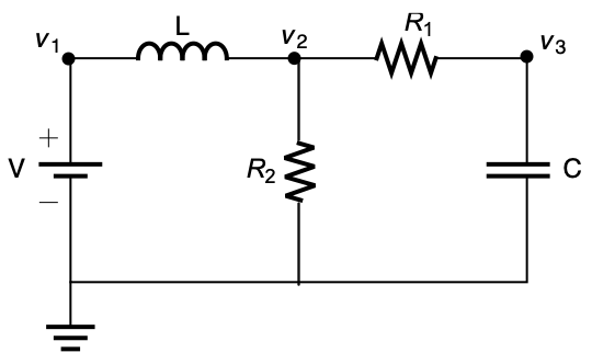
components2 = {r1 iR1[t] == vR1[t], l iL'[t] == vL[t], iC[t] == c vC'[t], r2 iR2[t] == vR2[t]};
connections2 = {vL[t] + vR2[t] == v1[t], vR1[t] + vC[t] == vR2[t], iL[t] == iR1[t] + iR2[t], iR1[t] == iC[t]};ic2 = {iR1[0] == 0, iR2[0] == 0, iL[0] == 0, iC[0] == 0, vR1[0] == 0, vR2[0] == 0, vL[0] == 0, vC[0] == 0};
params2 = {r1 -> 5, r2 -> 10, l -> 10 ^ -2, c -> 10 ^ -4};v1[t_] := UnitStep[t - .01];sol2 = NDSolve[{components2, connections2, ic2} /. params2, vC, {t, 0, .03}];Plot[Evaluate[{v1[t], vC[t]} /. sol2], {t, 0, .03}, Filling -> {1 -> 0}, Ticks -> {Range[0.01, 0.03, 0.01], Automatic}, PlotRange -> {0, 1.5}]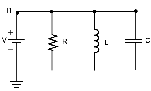
components = {r iR[t] == vR[t], l iL'[t] == vL[t], iC[t] == c vC'[t]};
connections = {iC[t] + iR[t] + iL[t] == i1[t], v[t] == vR[t], vR[t] == vL[t], vL[t] == vC[t]};i1[t_] := 1;ic = {v[0] == vR[0] == vR[0] == vC[0] == iR[0] == iL[0] == iC[0] == 0};
params = {r -> 10, c -> 10 ^ -3, l -> 0.4};
sol = NDSolve[{components, connections, iL[0] == 0, v[0] == 0} /. params, {iR, iL, iC, v}, {t, 0, 0.2}, AccuracyGoal -> 7];R,L,Cの各コンポーネントにおける電流とその結果の電圧を示す:
{Plot[Evaluate[{iR[t], iL[t], iC[t]} /. sol], {t, 0, 0.2}], Plot[v[t] /. sol, {t, 0, 0.2}]}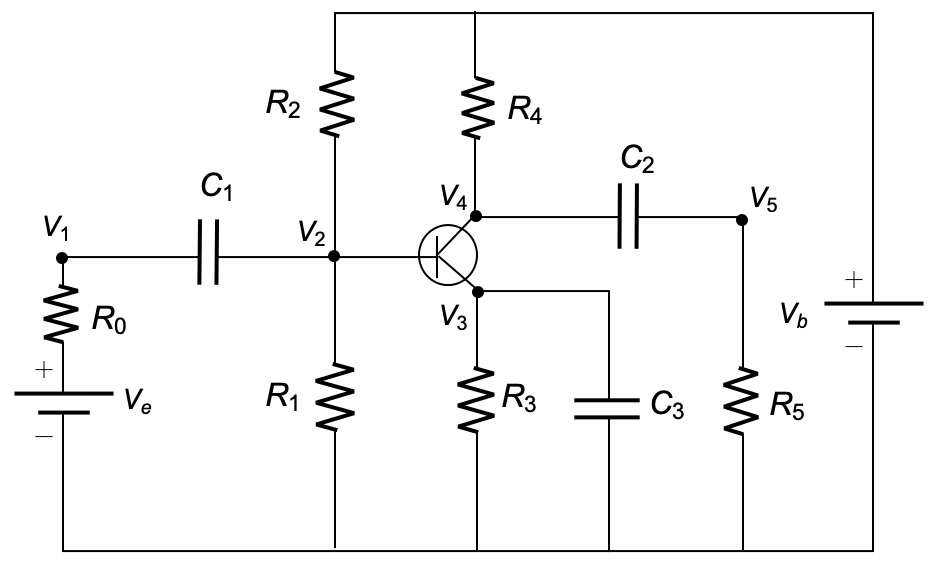

ve[t_] := (4 / 10) Sin[200 Pi t];
params = {vb -> 6, r0 -> 1000, r1 -> 9000, r2 -> 9000, r3 -> 9000, r4 -> 9000, r5 -> 9000, α -> 99 / 100, β -> 10 ^ -6, c1 -> 10 ^ -6, c2 -> 2 10 ^ -6, c3 -> 3 10 ^ -6};
v23[t_] = β (Exp[(v2[t] - v3[t]) / .026] - 1);オームの法則とキルヒッホフの法則を使って各ノードの支配方程式を求める:
node1 = c1 (v2'[t] - v1'[t]) == v1[t] / r0 - ve[t] / r0;
node2 = c1(v1'[t] - v2'[t]) == (1 - α)v23[t] + v2 [t] / r1 + v2[t] / r2 - vb / r2;
node3 = c2 v3'[t] == v23[t] - v3[t] / r3;
node4 = c3(v4'[t] - v5'[t]) == vb / r4 - v4[t] / r4 - α v23[t];
node5 = c3(v4'[t] - v5'[t]) == v5[t] / r5;
ics = {v1[0] == 0, v2[0] == vb / 2, v3[0] == vb / 2, v4[0] == vb, v5[0] == 0};sol = NDSolve[{node1, node2, node3, node4, node5, ics} /. params, {v1, v2, v3, v4, v5}, {t, 0, 0.2}, Method -> {"EquationSimplification" -> "Residual"}] ;

Plot[Evaluate[{v3[t], v4[t]} /. sol], {t, 0, 0.2}, PlotRange -> All]入力電圧レベル vi から希望する出力電圧レベル vd へのDC-DCブーストコンバータをパルス幅変調フィードバック制御 q[t]を使ってモデル化する:
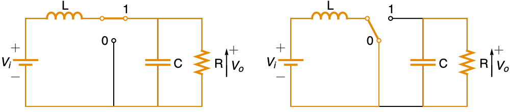
system = {vo'[t] == q[t]i[t] / c - vo[t] / (r c), i'[t] == -q[t]vo[t] / l + vi / l, vo[0] == 0, i[0] == 0};制御信号 q[t]が各周期 τ の vi/vd の割合でトランジスタをオンにする:
control = {q[0] == 1, WhenEvent[Mod[t, τ] == (vi / vd)τ, q[t] -> 0], WhenEvent[Mod[t, τ] == 0, q[t] -> 1]};pars = {vi -> 24, vd -> 36, r -> 22, l -> 2 10 ^ -1, c -> 1 10 ^ -4, τ -> 5 10 ^ -5};sol = NDSolve[{system, control} /. pars, {vo, i, q}, {t, 0, .2}, DiscreteVariables -> q];{Plot[{vo[t] /. sol, vd /. pars}, {t, 0, .2}, PlotRange -> All], Plot[q[t] /. sol, {t, 0, .0004}]}パルス幅変調フィードバック制御 q[t]を使って入力電圧レベル vi から希望する出力電圧レベルl vo へのDC-DC バックブーストコンバータをモデル化する:
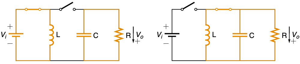
system = {i'[t] == q[t]vi / l - (1 - q[t])vo[t] / l , vo'[t] == i[t] / c - vo[t] / (r c), vo[0] == 0, i[0] == 0};制御信号 q[t]が各周期の vd/(vi+vd)の割合でトランジスタをオンにする:
control = {q[0] == 1, WhenEvent[Mod[t, τ] == (vd / (vi + vd))τ, q[t] -> 0], WhenEvent[Mod[t, τ] == 0, q[t] -> 1]};pars = {vi -> 24, vd -> 36, r -> 22, l -> 2 10 ^ -2, c -> 4 10 ^ -6, τ -> 5 10 ^ -5};sol = NDSolve[{system, control} /. pars, {vo, i, q}, {t, 0, .2}, DiscreteVariables -> q];{Plot[{vo[t] /. sol, vd /. pars}, {t, 0, .02}, PlotRange -> All], Plot[q[t] /. sol, {t, 0, .0004}]}pars = {vi -> 24, vd -> 16, r -> 22, l -> 2 10 ^ -2, c -> 4 10 ^ -6, τ -> 5 10 ^ -5};sol = NDSolve[{system, control} /. pars, {vo, i, q}, {t, 0, .2}, DiscreteVariables -> q];{Plot[{vo[t] /. sol, vd /. pars}, {t, 0, .02}, PlotRange -> All], Plot[q[t] /. sol, {t, 0, .0004}]}水力系 (3)
2本の円柱タンクがあり,水が一方のタンクからもう一方のタンクへとパイプを通って移動する.タンクの水面の高さの変化をモデル化する:
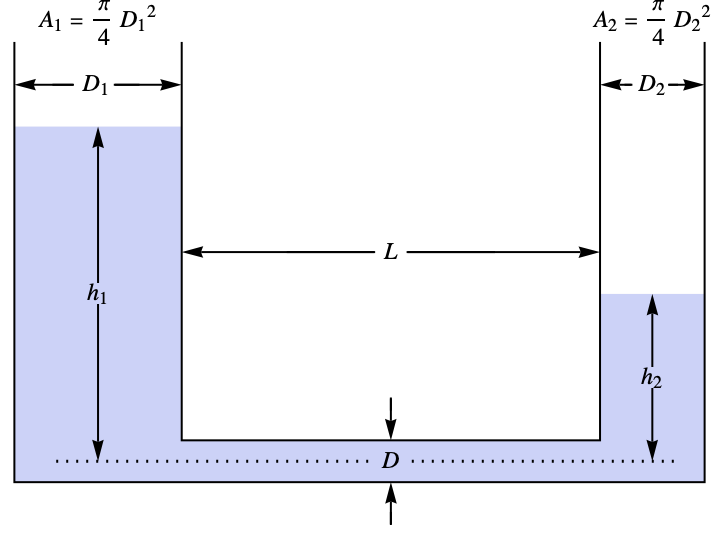
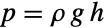
pressureEqns = {p1[t] == ρ g h1[t], p2[t] == ρ g h2[t]};
massConservation = {a1 h1'[t] == -flowRate, a2 h2'[t] == flowRate};Hagen–Poiseuilleの関係を使ってパイプを通る流れのシミュレーションを行う:
flowRate = (p1[t] - p2[t])(π pipeDia ^ 4) / (128 μ pipeLen);params = {pipeLen -> 0.1, pipeDia -> 0.2, ρ -> 0.2, μ -> 2 10 ^ -3, g -> 9.81};
{a1, a2} = {1, 1};sol = NDSolve[{pressureEqns, massConservation, h1[0] == 1, h2[0] == 0} /. params, {h1, h2, p1, p2}, {t, 0, 15}] ;Plot[Evaluate[{h1[t], h2[t]} /. sol], {t, 0, 15}, PlotRange -> All]massConservation = {a1 h1'[t] == -flowRate, a2 h2'[t] == flowRate - a2 h2[t] / 10};sol = NDSolve[{pressureEqns, massConservation, h1[0] == 1, h2[0] == 0} /. params, {h1, h2, p1, p2}, {t, 0, 80}] ;2番目のタンクの水漏れのために,両方のタンクがいずれ空になる:
Plot[Evaluate[{h1[t], h2[t]} /. sol], {t, 0, 80}, PlotRange -> All, AxesOrigin -> {0, 0}]パイプを通って片方のタンクからもう一方のタンクに水が流れる.この半円形の2つのタンクの水位変化をモデル化する:
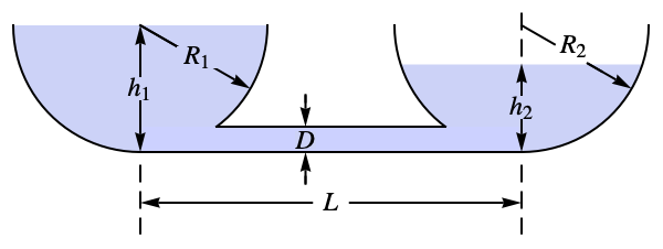
pressureEqns = {p1[t] == ρ g h1[t], p2[t] == ρ g h2[t]};
massConservation = {a1 h1'[t] == -flowRate, a2 h2'[t] == flowRate};flowRate = (p1[t] - p2[t])(π pipeDia ^ 4) / (128 μ pipeLen);
params = {pipeLen -> 0.1, pipeDia -> 0.2, ρ -> 0.2, μ -> 2 10 ^ -3, g -> 9.81};r1 = 1;r2 = 1;
hemisphereArea[r_, h_] := Pi (2 r h - h ^ 2);
a1 = hemisphereArea[r1, h1[t]];
a2 = hemisphereArea[r2, h2[t]];sol2 = NDSolve[{pressureEqns, massConservation, h1[0] == 1, h2[0] == 10 ^ -5} /. params, {h1, h2, p1, p2}, {t, 0, 15}] ;Plot[Evaluate[{h1[t], h2[t]} /. sol2], {t, 0, 15}, PlotRange -> All]1つのタンクが他の2つのタンクに水を供給する3つのタンクがある.この3つのタンクの水位変化をモデル化する:
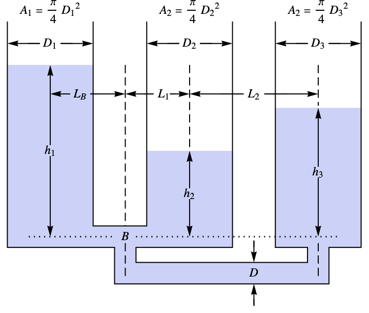
pressureEqns = {p1[t] == ρ g h1[t], p2[t] == ρ g h2[t], p3[t] == ρ g h3[t]};
massConservation = {a1 h1'[t] == -flowRate, a2 h2'[t] == flowRate1, a3 h3'[t] == flowRate2};Hagen–Poiseuille関係でパイプを通る水の流れをモデル化する:
flowRate = (p1[t] - pB[t])(π pipeDia ^ 4) / (128μ pipeLenB);
flowRate1 = (pB[t] - p2[t])(π pipeDia ^ 4) / (128μ pipeLen1);
flowRate2 = (pB[t] - p3[t])(π pipeDia ^ 4) / (128μ pipeLen2);
最初のタンクからの流量は他の2つのタンクの流量の和に等しい:
flowRateConstraint = flowRate == flowRate1 + flowRate2;params = {pipeLenB -> 0.1, pipeLen1 -> 0.1, pipeLen2 -> 0.2, pipeDia -> .2, ρ -> .2, μ -> 2 10 ^ -3, g -> 9.81};
{a1, a2, a3} = {1, 1, 1};sol = NDSolve[{pressureEqns, massConservation, flowRateConstraint, h1[0] == 1, h2[0] == 0, h3[0] == 0} /. params, {h1, h2, h3}, {t, 0, 15}];Plot[Evaluate[{h1[t], h2[t], h3[t]} /. sol], {t, 0, 15}, PlotRange -> All]massConservation = {a1 h1'[t] == -flowRate, a2 h2'[t] == flowRate1, a3 h3'[t] == flowRate2 - a3 h3[t] / 10};sol = NDSolve[{pressureEqns, massConservation, flowRateConstraint, h1[0] == 1, h2[0] == 0, h3[0] == 0} /. params, {h1, h2, h3}, {t, 0, 90}] ;Plot[Evaluate[{h1[t], h2[t], h3[t]} /. sol], {t, 0, 90}, PlotRange -> All]化学系 (2)
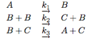
{r1, r2, r3} = {k1 a[t], k2 b[t] ^ 2, k3 b[t] c[t]};
eqns = {a'[t] == -r1 + r3, b'[t] == r1 - r2 - r3};eqEqn = {a[t] + b[t] + c[t] == 1};
icEqn = {a[0] == 1, b[0] == 0, c[0] == 0};params = {k1 -> 0.04, k2 -> 3 10 ^ 7, k3 -> 10 ^ 4};
sol = NDSolve[{eqns, eqEqn, icEqn} /. params, {a, b, c}, {t, 0, 10 ^ 8}];LogLinearPlot[Evaluate[#[t] /. sol], {t, 10 ^ -6, 10 ^ 8}, PlotRange -> All, PlotLabel -> #[t]]& /@ {a, b, c}二酸化炭素と連続的に混ざり合うFLBとZHUの2つの種の化学反応をモデル化する:
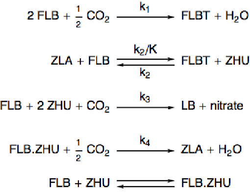
Fin = klA (pCO2 / H - CO2[t]);r1 = k1 FLB[t]^2CO2[t]^0.5;
r2 = k2 FLBT[t] ZHU[t];
r3 = (k2 / KK)FLB[t] ZLA[t];
r4 = k3 FLB[t]ZHU[t]^2 CO2[t];
r5 = k4 FLBZHU[t]CO2[t]^0.5;
eqns = {FLB'[t] == -2 r1 + r2 - r3 - r4, CO2'[t] == -0.5 r1 - r4 - 0.5r5 + Fin, FLBT'[t] == r1 - r2 + r3, ZHU'[t] == -r2 + r3 - 2 r4, ZLA'[t] == r2 - r3 + r5};eqEqn = Ks FLB[t] ZHU[t] == FLBZHU[t];方程式を解き,FLB,ZHU,CO2,ZLAの濃度の変化を求める:
params = {k1 -> 18.7, k2 -> 0.58, k3 -> 0.09, k4 -> 0.42, KK -> 34.4, klA -> 3.3, Ks -> 115.83, pCO2 -> 0.9, H -> 737};ic = {FLB[0] == 0.444, CO2[0] == 0.00123, FLBT[0] == 0, ZHU[0] == 0.007, ZLA[0] == 0};sol = NDSolve[{eqns, eqEqn, ic} /. params, {FLB, ZHU, CO2, ZLA}, {t, 0, 200}];Plot[Evaluate[#[t] /. sol], {t, 0, 200}, PlotRange -> All, PlotLabel -> #[t]]& /@ {FLB, ZHU, CO2, ZLA}特性と関係 (7)
DSolve[{y''[x] + y[x] == Cos[x], y[0] == y'[0] == 0}, y, x]NDSolve[{y''[x] + y[x] == Cos[x], y[0] == y'[0] == 0}, y, {x, 0, 20}]Plot[Evaluate[y[x] /. %], {x, 0, 20}]JacobiSNを定義する方程式:
NDSolve[{y'[x] ^ 2 == (1 - y[x] ^ 2)(1 - y[x] ^ 2 / 2), y[0] == 0}, y, {x, 0, 1.5}]Plot[Evaluate[y[x] /. %], {x, 0, 1.5}]Plot[JacobiSN[x, 1 / 2], {x, 0, 1.5}]iv = Table[{x, NIntegrate[Sin[Exp[s]], {s, 0, x}]}, {x, 0, 3, .25}]独立変数の関数では,NDSolveは実質的に不定積分を返す:
sol = NDSolve[{y'[x] == Sin[Exp[x]], y[0] == 0}, y, {x, 0, 3}]Plot[Evaluate[y[x] /. sol], {x, 0, 3}, Epilog -> Map[Point, iv]]ev[t_ ? NumberQ] := First[y[t] /. NDSolve[{y''[x] + y[x] == 0, y[0] == 1, y'[0] == 0}, y, {x, t}]]Plot[ev[t], {t, 0, 3}]FindRoot[ev[t], {t, 1}]NDSolve[{y''[x] + y[x] == 0, y[0] == 1, y'[0] == 0, WhenEvent[y[x] == 0, "StopIntegration"]}, y, {x, ∞}]

Subscript[y, 10][yp0_ ? NumberQ] := First[y[10] /. NDSolve[{y''[x] + Sin[y[x]] == 0, y[0] == 1, y'[0] == yp0}, y, {x, 10}]]Plot[Subscript[y, 10][Subsuperscript[y, 0, ′]], {Subsuperscript[y, 0, ′], -2, 2}]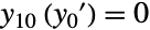
FindRoot[Subscript[y, 10][Subsuperscript[y, 0, ′]] == 0, {Subsuperscript[y, 0, ′], -1.5}]Plot[Evaluate[{y[x], y'[x]} /. NDSolve[{y''[x] + Sin[y[x]] == 0, y[0] == 1, y[10] == 0}, y, x]], {x, 0, 10}]NDSolveをSystemModelのソルバとして使う:
sim = SystemModelSimulate[[image], Method -> "NDSolve"]SystemModelPlot[sim, {"y", "z"}]SystemModelを使って大きい階層的モデルをモデル化する:
sim = SystemModelSimulate[[image]]SystemModelPlot[sim, {"tank1.h", "tank2.h", "tank3.h"}, PlotRange -> All]考えられる問題 (14)
NDSolveのメッセージの多くにはそのメッセージに特有の参照ページがある.各ページにアクセスする方法はワークフローのエラーメッセージを理解するを参照されたい.
数値誤差 (4)
NDSolve[{y''[x] + y[x] == 0, y[0] == 1, y'[0] == 0}, y, {x, 0, 100}]Plot[Evaluate[y[x] - Cos[x] /. %], {x, 0, 100}]NDSolve[{y''[x] == y[x](y[x] ^ 2 - 3 / 2), y[0] == 0, y'[0] == 1}, y, {x, 0, 10}]Plot[Evaluate[y[x] - JacobiSN[x, 1 / 2] /. %], {x, 0, 10}]高次のアルゴリズムでは,デフォルトの補間はステップ間で大きい誤差を生むことがある:
sol = NDSolve[{y''[x] == y[x](y[x] ^ 2 - 3 / 2), y[0] == 0, y'[0] == 1}, y, {x, 0, 10}, Method -> {"ExplicitRungeKutta", "DifferenceOrder" -> 8}]Plot[(y''[x] - y[x](y[x] ^ 2 - 3 / 2)) /. sol, {x, 0, 10}, PlotRange -> All]アルゴリズムに対応した次数の補間を使うとステップ間の誤差が小さくなる:
dsol = NDSolve[{y''[x] == y[x](y[x] ^ 2 - 3 / 2), y[0] == 0, y'[0] == 1}, y, {x, 0, 10}, Method -> {"ExplicitRungeKutta", "DifferenceOrder" -> 8}, InterpolationOrder -> All]Plot[(y''[x] - y[x](y[x] ^ 2 - 3 / 2)) /. dsol, {x, 0, 10}, PlotRange -> All]有限要素法が使うアルゴリズムの中には決定論的ではないものがある.このことは,このアルゴリズムの中で何らかの偶然性が使われ,同じ入力の実行結果に若干の差が出ることを意味する:
pdesolver := First[u /. NDSolve[{Laplacian[u[x, y], {x, y}] + 1 == 0, DirichletCondition[u[x, y] == 0, True]}, u, {x, 0, 1}, {y, 0, 1}]]同じ偏微分方程式を2度解く.2つの解には小さい差があるかもしれない:
MinMax[pdesolver["ValuesOnGrid"] - pdesolver["ValuesOnGrid"]]微分代数方程式 (3)
NDSolveは指数が1より大きい系を自動的には処理しない:
s = NDSolve[{x'''[t] + y[t] == Cos[t], x[t] == Sin[t], x[0] == 0, x'[0] == 1, x''[0] == 0}, {x, y}, {t, 0, 2 Pi}]
s = NDSolve[{x'''[t] + y[t] == Cos[t], x[t] == Sin[t], x[0] == 0, x'[0] == 1, x''[0] == 0}, {x, y}, {t, 0, 2 Pi}, Method -> {"IndexReduction" -> Automatic}]Plot[Evaluate[{x[t], y[t]} /. s], {t, 0, 2 Pi}]DAE = {Derivative[1][Subscript[x, 1]][t] == Subscript[x, 3][t], Subscript[x, 2][t] (1 - Subscript[x, 2][t]) == 0, Subscript[x, 1][t] Subscript[x, 2][t] + Subscript[x, 3][t] (1 - Subscript[x, 2][t]) == t};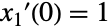
sol = NDSolve[{DAE, Subscript[x, 1]'[0] == 1}, {Subscript[x, 1], Subscript[x, 2], Subscript[x, 3]}, {t, 0, 1}]NDSolveは,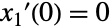 で解が求まらない場合は,指定された初期条件を変えることがある:
sol = NDSolve[{DAE, Subscript[x, 1]'[0] == 0}, {Subscript[x, 1], Subscript[x, 2], Subscript[x, 3]}, {t, 0, 1}]
Subscript[x, 1]'[0] /. solsol = NDSolve[{DAE, Subscript[x, 1]'[0] == 0}, {Subscript[x, 1], Subscript[x, 2], Subscript[x, 3]}, {t, 0, 1}, Method -> {"DAEInitialization" -> {"Collocation", "DefaultStartingValue" -> 0}}]NDSolveは指数1に限定されるが,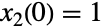 の解の指数は2である:
sol = NDSolve[{DAE, Subscript[x, 1][0] == 0, Subscript[x, 2][0] == 1, Subscript[x, 3][0] == 1}, {Subscript[x, 1], Subscript[x, 2], Subscript[x, 3]}, {t, 0, 1}]

高指数の系を解く場合は,指数減少法を使って微分代数方程式の指数を1にするとよい:
sol = NDSolve[{DAE, Subscript[x, 1][0] == 0, Subscript[x, 2][0] == 1, Subscript[x, 3][0] == 1}, {Subscript[x, 1], Subscript[x, 2], Subscript[x, 3]}, {t, 0, 1}, Method -> {"IndexReduction" -> True, "DAEInitialization" -> "Collocation"}]デフォルトのメソッドではデフォルトの許容度には収束できないかもしれない:
s = 100;
dae = {x'[t] == -(xs[t] - ys[t]), y'[t] == (xs[t] - ys[t]), xs[t] == s x[t], ys[t] == s y[t], x[0] == 1, y[0] == 0, xs[0] == s, ys[0] == 0};NDSolve[dae, {x, y}, {t, 0, 1}]
AccuracyGoalとPrecisionGoalの設定値を低くすると解が求まる:
NDSolve[dae, {x, y}, {t, 0, 1}, AccuracyGoal -> 6, PrecisionGoal -> 6]"StateSpace"時間積分法はデフォルトの許容度でこの問題を解くことができる:
NDSolve[dae, {x, y}, {t, 0, 1}, Method -> {"TimeIntegration" -> "StateSpace"}]偏微分方程式 (4)
PDEModelsの概要には,さまざまな分野からの詳細な説明付きのPDEモデルの大規模コレクションが収められている.
L = 20;
wpde = {Subscript[∂, t, t]u[t, x] == Subscript[∂, x, x]u[t, x] + (1 - u[t, x]^2) (1 + 2 u[t, x]), u[0, x] == E^-x^2, u^(1, 0)[0, x] == 0, u[t, -L] == u[t, L]};
空間的な離散化は初期値に基づいており,それは最終値に比べると変化が少ない:
s1 = NDSolve[wpde, u, {t, 0, L}, {x, -L, L}]
空間的な格子点の最小数を大きくすることで,最終値が正確に計算できるようになる:
s2 = NDSolve[wpde, u, {t, 0, 20}, {x, -L, L}, Method -> {"PDEDiscretization" -> {"MethodOfLines", "SpatialDiscretization" -> {"TensorProductGrid", "MinPoints" -> 750}}}]このプロットは,空間的により複雑な解のオンセットを示している:
DensityPlot[Evaluate[u[-t, x] /. First[s2]], {x, -L, L}, {t, 0, -L}, PlotPoints -> 50]hpde = {D[u[t, x], t] == D[u[t, x], x, x], u[0, x] == UnitStep[1 / 2 - x], u[t, 0] == 1, u[t, 1] == 0};初期値における不連続性によって空間格子点が多すぎるようになるかもしれない:
Plot3D[Evaluate[u[t, x] /. NDSolve[hpde, u, {t, 0, .01}, {x, 0, 1}]], {x, 0, 1}, {t, 0, .01}]
空間格子点の数をより少なく設定しても,基本的に同じような解になる:
Plot3D[Evaluate[u[t, x] /. NDSolve[hpde, u, {t, 0, .01}, {x, 0, 1}, Method -> {"PDEDiscretization" -> {"MethodOfLines", "SpatialDiscretization" -> {"TensorProductGrid", "MaxPoints" -> 100}}}]], {x, 0, 1}, {t, 0, .01}]
lpde = {D[u[x, y], x, x] + D[u[x, y], y, y] == 0, u[x, 0] == Sin[Pi x], Derivative[0, 1][u][x, 0] == 0, u[0, y] == u[1, y] == 0};このソルバは初期値(Cauchy)問題としてよく設定できた方程式にしか使えない:
sol = NDSolve[lpde, u, {x, 0, 1}, {y, 0, 1}]
Plot3D[Evaluate[u[x, y] /. sol], {x, 0, 1}, {y, 0, 1}, PlotRange -> All]境界値問題 (1)
Plot[Evaluate[{y[x], y'[x]} /. NDSolve[{y''[x] + Sin[y[x]] == 0, y[0] == 0, y[10] == 0}, y, x]], {x, 0, 10}]解の探索に開始条件を加えることで,他の解を求めることができる:
Table[Plot[Evaluate[{y[x], y'[x]} /. NDSolve[{y''[x] + Sin[y[x]] == 0, y[0] == 0, y[10] == 0}, y, x, Method -> {"BoundaryValues" -> {"Shooting", "StartingInitialConditions" -> {y[0] == 0, y'[0] == i}}}]], {x, 0, 10}], {i, 1, 2}]

 NKS|Online
テキスト
Wolfram Research (1991), NDSolve, Wolfram言語関数, https://reference.wolfram.com/language/ref/NDSolve.html (2019年に更新).
CMS
Wolfram Language. 1991. "NDSolve." Wolfram Language & System Documentation Center. Wolfram Research. Last Modified 2019. https://reference.wolfram.com/language/ref/NDSolve.html.
APA
Wolfram Language. (1991). NDSolve. Wolfram Language & System Documentation Center. Retrieved from https://reference.wolfram.com/language/ref/NDSolve.html