SemidefiniteOptimization[c,{a0,a1,…,ak}]
finds a vector ![]() that minimizes the quantity
that minimizes the quantity ![]() subject to the linear matrix inequality constraint
subject to the linear matrix inequality constraint ![]() .
.


SemidefiniteOptimization
SemidefiniteOptimization[f,cons,vars]
finds values of variables vars that minimize the linear objective f subject to semidefinite constraints cons.
SemidefiniteOptimization[c,{a0,a1,…,ak}]
finds a vector ![]() that minimizes the quantity
that minimizes the quantity ![]() subject to the linear matrix inequality constraint
subject to the linear matrix inequality constraint ![]() .
.
SemidefiniteOptimization[…,"prop"]
specifies what solution property "prop" should be returned.
Details and Options
- SemidefiniteOptimization is also known as semidefinite programming (SDP) and mixed-integer semidefinite programming (MISDP).
- Semidefinite optimization is a convex optimization problem that can be solved globally and efficiently with real, integer or complex variables.
- Semidefinite optimization finds
 that solves the primal problem:
 -
minimize 
subject to constraints ![a_(0)+a_(1) x_(1)+...+a_(k) x_(k)>=_(TemplateBox[{n}, SemidefiniteConeList])0](Files/SemidefiniteOptimization.en/6.png "a_(0)+a_(1) x_(1)+...+a_(k) x_(k)>=_(TemplateBox[{n}, SemidefiniteConeList])0")
where 
- The matrices
 must be symmetric
  matrices.
 - Mixed-integer semidefinite optimization finds
 and
and  that solve the problem:
 -
minimize 
subject to constraints ![a_(0)+a_(1) x_(1)+...+a_(k_r) x_(k_r)+a_(k_r+1)y_1+...+a_(k_r+k_i)y_(k_i)>=_(TemplateBox[{n}, SemidefiniteConeList])0](Files/SemidefiniteOptimization.en/13.png "a_(0)+a_(1) x_(1)+...+a_(k_r) x_(k_r)+a_(k_r+1)y_1+...+a_(k_r+k_i)y_(k_i)>=_(TemplateBox[{n}, SemidefiniteConeList])0")
where 
- When the objective function is real valued, SemidefiniteOptimization solves problems with
![x in TemplateBox[{}, Complexes]^n](Files/SemidefiniteOptimization.en/15.png "x in TemplateBox[{}, Complexes]^n") by internally converting to real variables
by internally converting to real variables  , where
  and
and  . Linear matrix inequalities may be specified with Hermitian matrices
  .
. - The variable specification vars should be a list with elements giving variables in one of the following forms:
-
v variable with name  and dimensions inferred
v∈Reals real scalar variable v∈Integers integer scalar variable v∈Complexes complex scalar variable v∈ℛ vector variable restricted to the geometric region 
v∈Vectors[n,dom] vector variable in  or
or 
v∈Matrices[{m,n},dom] matrix variable in  or
or 
- The constraints cons can be specified by:
-
LessEqual 
scalar inequality GreaterEqual 
scalar inequality VectorLessEqual 
vector inequality VectorGreaterEqual 
vector inequality Equal 
scalar or vector equality Element 
convex domain or region element - With SemidefiniteOptimization[f,cons,vars], parameter equations of the form parval, where par is not in vars and val is numerical or an array with numerical values, may be included in the constraints to define parameters used in f or cons. »
- The primal minimization problem has a related maximization problem that is the Lagrangian dual problem. The dual maximum value is always less than or equal to the primal minimum value, so it provides a lower bound. The dual maximizer provides information about the primal problem, including sensitivity of the minimum value to changes in the constraints. »
- The semidefinite optimization has a dual: »
-
maximize ![-TemplateBox[{Tr, paclet:ref/Tr}, RefLink, BaseStyle -> {2ColumnTableMod}][a_0.lambda]](Files/SemidefiniteOptimization.en/33.png "-TemplateBox[{Tr, paclet:ref/Tr}, RefLink, BaseStyle -> {2ColumnTableMod}][a_0.lambda]")
subject to constraints ![TemplateBox[{Tr, paclet:ref/Tr}, RefLink, BaseStyle -> {2ColumnTableMod}][a_j.lambda]=c_j,j=1,..., k,lambda>=_(TemplateBox[{n}, SemidefiniteConeList])0](Files/SemidefiniteOptimization.en/34.png "TemplateBox[{Tr, paclet:ref/Tr}, RefLink, BaseStyle -> {2ColumnTableMod}][a_j.lambda]=c_j,j=1,..., k,lambda>=_(TemplateBox[{n}, SemidefiniteConeList])0")
where 
- The possible solution properties "prop" include:
-
"PrimalMinimizer" 
a list of variable values that minimizes the objective function "PrimalMinimizerRules" 
values for the variables vars={v1,…} that minimize 
"PrimalMinimizerVector" 
the vector that minimizes 
"PrimalMinimumValue" 
the primal minimum value 
"DualMaximizer" 
the matrix that maximizes ![-TemplateBox[{Tr, paclet:ref/Tr}, RefLink, BaseStyle -> {3ColumnTableMod}][a_0.lambda]](Files/SemidefiniteOptimization.en/44.png "-TemplateBox[{Tr, paclet:ref/Tr}, RefLink, BaseStyle -> {3ColumnTableMod}][a_0.lambda]")
"DualMaximumValue" ![-TemplateBox[{Tr, paclet:ref/Tr}, RefLink, BaseStyle -> {3ColumnTableMod}][a_0.lambda^*]](Files/SemidefiniteOptimization.en/45.png "-TemplateBox[{Tr, paclet:ref/Tr}, RefLink, BaseStyle -> {3ColumnTableMod}][a_0.lambda^*]")
the dual maximum value "DualityGap" ![-TemplateBox[{Tr, paclet:ref/Tr}, RefLink, BaseStyle -> {3ColumnTableMod}][a_0.lambda^*] - c.x^*](Files/SemidefiniteOptimization.en/46.png "-TemplateBox[{Tr, paclet:ref/Tr}, RefLink, BaseStyle -> {3ColumnTableMod}][a_0.lambda^*] - c.x^*")
the difference between the dual and primal optimal values "Slack" 
matrix that converts inequality constraints to equality "ConstraintSensitivity" 
sensitivity of  to constraint perturbations
"ObjectiveVector" 
the linear objective vector "ConstraintMatrices" 
the list of constraint matrices {"prop1","prop2",…} several solution properties - The following options may be given:
-
MaxIterations Automatic maximum number of iterations to use Method Automatic the method to use PerformanceGoal $PerformanceGoal aspects of performance to try to optimize Tolerance Automatic the tolerance to use for internal comparisons - The option Method->method may be used to specify the method to use. Available methods include:
-
Automatic choose the method automatically "CSDP" CSDP semidefinite optimization solver "DSDP" DSDP semidefinite optimization solver "SCS" SCS splitting conic solver "MOSEK" Commercial MOSEK convex optimization solver - Computations are limited to MachinePrecision.
Examples
open all close allBasic Examples (3)
Minimize ![]() subject to the linear matrix inequality constraint
subject to the linear matrix inequality constraint ![]() :
:
Subscript[a, 0] = (| | |
| - | - |
| 0 | 1 |
| 1 | 0 |);Subscript[a, 1] = (| | |
| - | - |
| 1 | 0 |
| 0 | 0 |);Subscript[a, 2] = (| | |
| - | - |
| 0 | 0 |
| 0 | 1 |);
res = SemidefiniteOptimization[2Subscript[x, 1] + 3Subscript[x, 2], Subscript[a, 0] + Subscript[a, 1]Subscript[x, 1] + Subscript[a, 2] Subscript[x, 2]Underscript[, {"SemidefiniteCone", 2}]0, {Subscript[x, 1], Subscript[x, 2]}]The optimal point is where ![]() is smallest within the region defined by the constraints:
is smallest within the region defined by the constraints:
Show[Plot3D[2Subscript[x, 1] + 3Subscript[x, 2], {Subscript[x, 1], Subscript[x, 2]}∈ImplicitRegion[Subscript[x, 1]Subscript[x, 2] - 1 ≥ 0 && Subscript[x, 1] ≥ 0 && Subscript[x, 2] ≥ 0, {Subscript[x, 1], Subscript[x, 2]}], ...], Graphics3D[{Blue, PointSize[0.04], Point[{Subscript[x, 1], Subscript[x, 2], 2Subscript[x, 1] + 3Subscript[x, 2]} /. res]}]]Minimize ![]() subject to the linear matrix inequality constraint
subject to the linear matrix inequality constraint ![]() :
:
Subscript[a, 0] = (| | |
| - | - |
| 0 | 1 |
| 1 | 0 |);Subscript[a, 1] = (| | |
| - | - |
| 1 | 0 |
| 0 | 0 |);Subscript[a, 2] = (| | |
| - | - |
| 0 | 0 |
| 0 | 1 |);
res = SemidefiniteOptimization[2Subscript[x, 1] + 3Subscript[x, 2], Subscript[a, 0] + Subscript[a, 1]Subscript[x, 1] + Subscript[a, 2]Subscript[x, 2]Underscript[, {"SemidefiniteCone", 2}]0, {Subscript[x, 1], Subscript[x, 2]}]Use the equivalent formulation with the objective vector and constraint matrices:
xmin = SemidefiniteOptimization[{2, 3}, {Subscript[a, 0], Subscript[a, 1], Subscript[a, 2]}]Subscript[a, 0] = (| | |
| - | - |
| 0 | 1 |
| 1 | 0 |);Subscript[a, 1] = (| | |
| - | - |
| 1 | 0 |
| 0 | 0 |);Subscript[a, 2] = (| | |
| - | - |
| 0 | 0 |
| 0 | 1 |);
SemidefiniteOptimization[2Subscript[x, 1] + 3Subscript[x, 2], Subscript[a, 0] + Subscript[a, 1]Subscript[x, 1] + Subscript[a, 2]Subscript[x, 2]Underscript[, {"SemidefiniteCone", 2}]0, {Subscript[x, 1]∈Integers,
Subscript[x, 2]∈Reals}]Use the equivalent formulation with the objective vector and constraint matrices:
SemidefiniteOptimization[{2, 3}, {Subscript[a, 0], Subscript[a, 1], Subscript[a, 2]}, {Integers, Reals}]Scope (29)
Basic Uses (13)
Minimize ![]() subject to constraints
subject to constraints ![]() :
:
res = SemidefiniteOptimization[x + 2y, {x^2 + 2y^2 ≤ 3, x + y == 2, x ≥ 1}, {x, y}]Minimize ![]() when the matrix
when the matrix ![]() is positive semidefinite:
is positive semidefinite:
constraint = VectorGreaterEqual[{{{x, 1}, {1, y}}, 0}, {"SemidefiniteCone", 2}]SemidefiniteOptimization[x + y, constraint, {x, y}]Minimize ![]() subject to the linear matrix inequality constraint
subject to the linear matrix inequality constraint ![]() :
:
c = {1, 1};Subscript[a, 0] = (| | |
| -- | -- |
| 0 | -1 |
| -1 | 0 |);Subscript[a, 1] = (| | |
| - | - |
| 1 | 1 |
| 1 | 1 |);Subscript[a, 2] = (| | |
| - | -- |
| 1 | 0 |
| 0 | -1 |);SemidefiniteOptimization[c.{x, y}, Subscript[a, 0] + Subscript[a, 1]x + Subscript[a, 2]yUnderscript[, {"SemidefiniteCone", 2}]0, {x, y}]The left-hand side of the constraint can be given in evaluated form:
Subscript[a, 0] + Subscript[a, 1]x + Subscript[a, 2]y//MatrixFormSemidefiniteOptimization[x + y, (| | |
| ------ | ------ |
| x + y | -1 + x |
| -1 + x | x - y |)Underscript[, {"SemidefiniteCone", 2}]0, {x, y}]Express the problem with the objective vector and constraint matrices:
SemidefiniteOptimization[c, {Subscript[a, 0], Subscript[a, 1], Subscript[a, 2]}]c = {1, 2};Subscript[a, 0] = (| | |
| - | - |
| 0 | 1 |
| 1 | 0 |);Subscript[a, 1] = (| | |
| - | - |
| 1 | 0 |
| 0 | 0 |);Subscript[a, 2] = (| | |
| - | - |
| 0 | 0 |
| 0 | 1 |);SemidefiniteOptimization[c.v, {Subscript[a, 1], Subscript[a, 2]}.vUnderscript[, {"SemidefiniteCone", 2}]-Subscript[a, 0], v]Use a vector variable ![]() and Inactive[Plus] to avoid unintended threading:
and Inactive[Plus] to avoid unintended threading:
c = {1, 2};Subscript[a, 0] = (| | |
| - | - |
| 0 | 1 |
| 1 | 0 |);Subscript[a, 1] = (| | |
| - | - |
| 1 | 0 |
| 0 | 0 |);Subscript[a, 2] = (| | |
| - | - |
| 0 | 0 |
| 0 | 1 |);SemidefiniteOptimization[c.v, Subscript[a, 0] + {Subscript[a, 1], Subscript[a, 2]}.vUnderscript[, {"SemidefiniteCone", 2}]0, v]Use a vector variable ![]() and parameter equations to avoid unintended threading:
and parameter equations to avoid unintended threading:
parEqs = {Subscript[a, 0] == (| | |
| - | - |
| 0 | 1 |
| 1 | 0 |), Subscript[a, 1] == (| | |
| - | - |
| 1 | 0 |
| 0 | 0 |), Subscript[a, 2] == (| | |
| - | - |
| 0 | 0 |
| 0 | 1 |)};SemidefiniteOptimization[{1, 2}.v, {parEqs, Subscript[a, 0] + {Subscript[a, 1], Subscript[a, 2]}.vUnderscript[, {"SemidefiniteCone", 2}]0}, v]Use a vector variable ![]() and Indexed[x,i] to specify individual components:
and Indexed[x,i] to specify individual components:
SemidefiniteOptimization[{1, 2}.x, (| | |
| --------------- | --------------- |
| Indexed[x, {1}] | 1 |
| 1 | Indexed[x, {2}] |)Underscript[, {"SemidefiniteCone", 2}]0, x]Use Vectors[n] to specify the dimension of a vector variable when it is ambiguous:
SemidefiniteOptimization[Indexed[x, {1}] + 2Indexed[x, {2}], (| | |
| --------------- | --------------- |
| Indexed[x, {1}] | 1 |
| 1 | Indexed[x, {2}] |)Underscript[, {"SemidefiniteCone", 2}]0, x]SemidefiniteOptimization[Indexed[x, {1}] + Indexed[2x, {2}], (| | |
| --------------- | --------------- |
| Indexed[x, {1}] | 1 |
| 1 | Indexed[x, {2}] |)Underscript[, {"SemidefiniteCone", 2}]0, x∈Vectors[2]]Several linear inequality constraints can be expressed with VectorGreaterEqual:
SemidefiniteOptimization[x + y, VectorGreaterEqual[{{x + 2y, x + 1}, {3, -1}}], {x, y}]Use ![]() v>=
v>=![]() or \[VectorGreaterEqual] to enter the vector inequality sign :
or \[VectorGreaterEqual] to enter the vector inequality sign :
SemidefiniteOptimization[x + y, {x + 2y, x}{3, -1}, {x, y}]An equivalent form using scalar inequalities:
SemidefiniteOptimization[x + y, {x + 2y ≥ 3, x ≥ -1}, {x, y}]Use a vector variable ![]() and vector inequality:
and vector inequality:
SemidefiniteOptimization[{1, 1}.v, {{1, 2}, {1, 0}}.v{3, -1}, v]Specify non-negative constraints using NonNegativeReals (![]() ):
):
SemidefiniteOptimization[{1, 1}.v, {1, 2}.v3, v∈Vectors[2, NonNegativeReals]]An equivalent form using vector inequalities:
SemidefiniteOptimization[{1, 1}.v, {{{1, 2}, {1, 0}}.v{3, 0}, v0}, v]Second-order cone constraints of the form ![]() can be used:
can be used:
SemidefiniteOptimization[{1, 1}.x, Norm[x] ≤ 1, x]"NormCone" constraints of the form ![]() can be used:
can be used:
constraint = VectorGreaterEqual[{{x, y, 3}, 0}, {"NormCone", 3}]SemidefiniteOptimization[x + y, constraint, {x, y}]Integer Variables (4)
Specify integer domain constraints using Integers:
SemidefiniteOptimization[x + y, {x + 2y ≥ 3, x ≥ -2}, {x∈Integers, y∈Integers}]Specify integer domain constraints on vector variables using Vectors[n,Integers]:
SemidefiniteOptimization[Total[x], {a == {{1, 2}, {1, 0}}, b == {3, -2},
a.xb}, {x∈Vectors[2, Integers]}]Specify non-negative integer domain constraints using NonNegativeIntegers (![]() ):
):
SemidefiniteOptimization[x + 2y, {x^2 + 2y^2 ≤ 3, x + y == 2, x∈NonNegativeIntegers}, {x, y}]Specify non-positive integer domain constraints using NonPositiveIntegers (![]() ):
):
SemidefiniteOptimization[-x + y, {x + 2y ≥ 3, x∈NonPositiveIntegers}, {x, y}]Complex Variables (2)
Specify complex variables using Complexes:
SemidefiniteOptimization[Re[z] + Im[z], Abs[z] ≤ 2, z∈Complexes]In linear matrix inequalities, the constraint matrices can be Hermitian or real symmetric:
Subscript[a, 0] = (| | |
| ----- | ----- |
| 0 | 1 + I |
| 1 - I | 0 |);Subscript[a, 1] = (| | |
| - | - |
| 1 | 0 |
| 0 | 0 |);Subscript[a, 2] = (| | |
| - | - |
| 0 | 0 |
| 0 | 1 |);The variables in linear matrix inequalities need to be real for the sum to remain Hermitian:
c = {1, 2};
SemidefiniteOptimization[c.v, {Subscript[a, 1], Subscript[a, 2]}.vUnderscript[, {"SemidefiniteCone", 2}]-Subscript[a, 0], v∈Vectors[2, Reals]]Primal Model Properties (3)
Minimize the function ![]() subject to the constraint
subject to the constraint ![]() :
:
SemidefiniteOptimization[x + y, (| | |
| - | - |
| x | 1 |
| 1 | y |)Underscript[, {"SemidefiniteCone", 2}]0, {x, y}]Get the primal minimizer as a vector:
{xmin, ymin} = SemidefiniteOptimization[x + y, (| | |
| - | - |
| x | 1 |
| 1 | y |)Underscript[, {"SemidefiniteCone", 2}]0, {x, y}, "PrimalMinimizer"]minval = SemidefiniteOptimization[x + y, (| | |
| - | - |
| x | 1 |
| 1 | y |)Underscript[, {"SemidefiniteCone", 2}]0, {x, y}, "PrimalMinimumValue"]Show[Plot3D[x + y, {x, y}∈ImplicitRegion[x y ≥ 1, {{x, 0, 5}, {y, 0, 5}}], MeshFunctions -> {#3&}], Graphics3D[{Red, PointSize[0.05], Point[{xmin, ymin, minval}]}]]c = SemidefiniteOptimization[x + y, (| | |
| - | - |
| x | 1 |
| 1 | y |)Underscript[, {"SemidefiniteCone", 2}]0, {x, y}, "ObjectiveVector"]Extract the constraint matrices:
mats = SemidefiniteOptimization[x + y, (| | |
| - | - |
| x | 1 |
| 1 | y |)Underscript[, {"SemidefiniteCone", 2}]0, {x, y}, "ConstraintMatrices"];Map[MatrixForm, mats]Use the extracted objective vector and constraint matrices for direct input:
SemidefiniteOptimization[c, mats]The slack for an inequality ![]() at the minimizer
at the minimizer ![]() is given by
is given by ![]() :
:
s = SemidefiniteOptimization[Subscript[x, 1] + 2Subscript[x, 2], (| | |
| -- | -- |
| x1 | 1 |
| 1 | x2 |)Underscript[, {"SemidefiniteCone", 2}]0, {Subscript[x, 1], Subscript[x, 2]}, "Slack"]//NormalExtract the minimizer and constraint matrices:
{x^ * , a} = SemidefiniteOptimization[Subscript[x, 1] + 2Subscript[x, 2],
(| | |
| -- | -- |
| x1 | 1 |
| 1 | x2 |)Underscript[, {"SemidefiniteCone", 2}]0, {Subscript[x, 1], Subscript[x, 2]}, {"PrimalMinimizer", "ConstraintMatrices"}]//NormalVerify that the slack matrix satisfies ![]() :
:
Prepend[x^ * , 1].a - sDual Model Properties (3)
c = {2, 3};Subscript[a, 0] = (| | |
| - | - |
| 0 | 1 |
| 1 | 0 |);Subscript[a, 1] = (| | |
| - | - |
| 1 | 0 |
| 0 | 0 |);Subscript[a, 2] = (| | |
| - | - |
| 0 | 0 |
| 0 | 1 |);
xv = Table[Indexed[x, i], {i, 2}];psol = SemidefiniteOptimization[c.xv, Subscript[a, 0] + {Subscript[a, 1], Subscript[a, 2]}.xvUnderscript[, {"SemidefiniteCone", 2}]0, xv]The dual problem is to maximize ![]() subject to
subject to ![]() :
:
constraints = {Table[Tr[Subscript[a, i].y] == c[[i]], {i, 2}], yUnderscript[, {"SemidefiniteCone", 2}]0};dsol = SemidefiniteOptimization[Tr[Subscript[a, 0].y], constraints, y∈Matrices[2]]The primal minimum value and the dual maximum value coincide because of strong duality:
{c.xv /. psol, -Tr[Subscript[a, 0].y] /. dsol}That is the same as having a duality gap of zero. In general, ![]() at optimal points:
at optimal points:
SemidefiniteOptimization[c.xv, Subscript[a, 0] + {Subscript[a, 1], Subscript[a, 2]}.xvUnderscript[, {"SemidefiniteCone", 2}]0, xv, "DualityGap"]Construct the dual problem using constraint matrices extracted from the primal problem:
obj = 2x + 3y;
constraints = (| | |
| - | - |
| x | 1 |
| 1 | y |)Underscript[, {"SemidefiniteCone", 2}]0;SemidefiniteOptimization[obj, constraints, {x, y}]Extract the objective vector and constraint matrices:
{c, a} = SemidefiniteOptimization[obj, constraints, {x, y}, {"ObjectiveVector", "ConstraintMatrices"}];The dual problem is to maximize ![]() subject to
subject to ![]() :
:
SemidefiniteOptimization[Tr[a[[1]].y], {Table[Tr[a[[i + 1]].y] == c[[i]], {i, 2}], yUnderscript[, {"SemidefiniteCone", 2}]0}, y∈Matrices[2]]Get the dual maximum value and dual maximizer directly using solution properties:
obj = 2x + 3y;
constraints = (| | |
| - | - |
| x | 1 |
| 1 | y |)Underscript[, {"SemidefiniteCone", 2}]0;SemidefiniteOptimization[obj, constraints, {x, y}, "DualMaximumValue"]The "DualMaximizer" can be obtained with:
SemidefiniteOptimization[obj, constraints, {x, y}, "DualMaximizer"]//NormalSensitivity Properties (4)
Use "ConstraintSensitivity" to find the change in optimal value due to constraint perturbations:
c = {2, 3};Subscript[a, 0] = (| | |
| - | - |
| 0 | 3 |
| 3 | 0 |);Subscript[a, 1] = (| | |
| - | - |
| 1 | 0 |
| 0 | 0 |);Subscript[a, 2] = (| | |
| - | - |
| 0 | 0 |
| 0 | 1 |);p^ * = SemidefiniteOptimization[c, {Subscript[a, 0], Subscript[a, 1], Subscript[a, 2]}, "PrimalMinimumValue"]sens = SemidefiniteOptimization[c, {Subscript[a, 0], Subscript[a, 1], Subscript[a, 2]}, "ConstraintSensitivity"]//NormalConsider new constraints ![]() where
where ![]() is the perturbation:
is the perturbation:
δ = 0.01 * {{1, 2}, {2, 3}};The approximate new optimal value is:
p^ * + Tr[δ.sens]Compare to directly solving the perturbed problem:
SemidefiniteOptimization[c, {Subscript[a, 0] + δ, Subscript[a, 1], Subscript[a, 2]}, "PrimalMinimumValue"]The optimal value changes according to the signs of the sensitivity matrix elements:
c = {2, 3};Subscript[a, 0] = (| | |
| - | - |
| 0 | 3 |
| 3 | 0 |);Subscript[a, 1] = (| | |
| - | - |
| 1 | 0 |
| 0 | 0 |);Subscript[a, 2] = (| | |
| - | - |
| 0 | 0 |
| 0 | 1 |);{p^ * , sens} = SemidefiniteOptimization[c, {Subscript[a, 0], Subscript[a, 1], Subscript[a, 2]}, {"PrimalMinimumValue", "ConstraintSensitivity"}];sens//NormalAt negative sensitivity element position, a positive perturbation will decrease the optimal value:
p^ * > SemidefiniteOptimization[c, {Subscript[a, 0] + {{0.01, 0}, {0, 0}}, Subscript[a, 1], Subscript[a, 2]}, "PrimalMinimumValue"]At positive sensitivity element position, a positive perturbation will increase the optimal value:
p^ * < SemidefiniteOptimization[c, {Subscript[a, 0] + {{0, 0.01}, {0.01, 0}}, Subscript[a, 1], Subscript[a, 2]}, "PrimalMinimumValue"]Express the perturbed constraints symbolically using Sylvester's criterion for semidefiniteness:
c = {2, 3};Subscript[a, 0] = (| | |
| - | - |
| 0 | 3 |
| 3 | 0 |);Subscript[a, 1] = (| | |
| - | - |
| 1 | 0 |
| 0 | 0 |);Subscript[a, 2] = (| | |
| - | - |
| 0 | 0 |
| 0 | 1 |);parameters = (| | |
| ----- | ----- |
| p1, 1 | p1, 2 |
| p1, 2 | p2, 2 |);matrix = Subscript[a, 0] + parameters + Subscript[x, 1]Subscript[a, 1] + Subscript[x, 2]Subscript[a, 2];
constraints = {matrix[[1, 1]] ≥ 0, matrix[[2, 2]] ≥ 0, Det[matrix] ≥ 0}With this form, the minimum value can be found exactly as a function of the parameters around 0:
Assuming[-1 < Subscript[p, 1, 2] < 1, exact = Refine[MinValue[2Subscript[x, 1] + 3Subscript[x, 2],
	{Subscript[x, 1] + Subscript[p, 1, 1] ≥ 0, Subscript[x, 2] + Subscript[p, 2, 2] ≥ 0, -1 + Subscript[x, 1]Subscript[x, 2] + Subscript[x, 2]Subscript[p, 1, 1] - 2Subscript[p, 1, 2] - Subsuperscript[p, 1, 2, 2] + Subscript[x, 1]Subscript[p, 2, 2] + Subscript[p, 1, 1]Subscript[p, 2, 2] ≥ 0}, {Subscript[x, 1], Subscript[x, 2]}]]]
Make a symmetric matrix with the derivatives of the minimum with respect to the parameters:
MatrixForm[N[smat = (| | |
| -------------------- | -------------------- |
| D[exact, p1, 1] | (1/2)D[exact, p1, 2] |
| (1/2)D[exact, p1, 2] | D[exact, p2, 2] |)]]This is the sensitivity to perturbation given by the "ConstraintSensitivity" property:
SemidefiniteOptimization[{2, 3}, {Subscript[a, 0], Subscript[a, 1], Subscript[a, 2]}, "ConstraintSensitivity"]//MatrixFormThe constraint sensitivity can also be obtained as the negative of the dual maximizer:
c = {2, 3};Subscript[a, 0] = (| | |
| - | - |
| 0 | 3 |
| 3 | 0 |);Subscript[a, 1] = (| | |
| - | - |
| 1 | 0 |
| 0 | 0 |);Subscript[a, 2] = (| | |
| - | - |
| 0 | 0 |
| 0 | 1 |);-SemidefiniteOptimization[c, {Subscript[a, 0], Subscript[a, 1], Subscript[a, 2]}, "DualMaximizer"]//MatrixFormSemidefiniteOptimization[c, {Subscript[a, 0], Subscript[a, 1], Subscript[a, 2]}, "ConstraintSensitivity"]//MatrixFormOptions (8)
Method (5)
The default method "CSDP" is an interior point method:
SemidefiniteOptimization[Subscript[x, 1] + Subscript[x, 2], (| | |
| -- | -- |
| x1 | 1 |
| 1 | x2 |)Underscript[, {"SemidefiniteCone", n}]0, {Subscript[x, 1], Subscript[x, 2]}, Method -> Automatic]SemidefiniteOptimization[Subscript[x, 1] + Subscript[x, 2], (| | |
| -- | -- |
| x1 | 1 |
| 1 | x2 |)Underscript[, {"SemidefiniteCone", n}]0, {Subscript[x, 1], Subscript[x, 2]}, Method -> "CSDP"]"DSDP" is an alternative interior point method:
SemidefiniteOptimization[Subscript[x, 1] + Subscript[x, 2], (| | |
| -- | -- |
| x1 | 1 |
| 1 | x2 |)Underscript[, {"SemidefiniteCone", n}]0, {Subscript[x, 1], Subscript[x, 2]}, Method -> "DSDP"]"SCS" uses a splitting conic solver method:
SemidefiniteOptimization[Subscript[x, 1] + Subscript[x, 2], (| | |
| -- | -- |
| x1 | 1 |
| 1 | x2 |)Underscript[, {"SemidefiniteCone", n}]0, {Subscript[x, 1], Subscript[x, 2]}, Method -> "SCS"]Different methods have different default tolerances, which affects the accuracy and precision:
{obj, cons, var} = {Subscript[x, 1] + Subscript[x, 2], (| | |
| -- | -- |
| x1 | 1 |
| 1 | x2 |)Underscript[, {"SemidefiniteCone", 2}]0, {Subscript[x, 1], Subscript[x, 2]}};Compute exact and approximate solutions:
{minval, argmin} = Minimize[obj, cons, var];
exact = {minval, var /. argmin}solCSDP = SemidefiniteOptimization[obj, cons, var, {"PrimalMinimumValue", "PrimalMinimizer"}, Method -> "CSDP"];solDSDP = SemidefiniteOptimization[obj, cons, var, {"PrimalMinimumValue", "PrimalMinimizer"}, Method -> "DSDP"];solSCS = SemidefiniteOptimization[obj, cons, var, {"PrimalMinimumValue", "PrimalMinimizer"}, Method -> "SCS"];"CSDP" and "DSDP" have default tolerances of ![]() :
:
solCSDP - exactsolDSDP - exact"SCS" has a default tolerance of ![]() :
:
solSCS - exactWhen the default method "CSDP" produces a message, try "DSDP" first:
a = {{{0, 2}, {2, 0}}, {{1, 2}, {2, 3}}, {{5, 0}, {0, 1}}};
c = {2, 3};{xmin, min} = SemidefiniteOptimization[c, a, {"PrimalMinimizer", "PrimalMinimumValue"}, Method -> "CSDP"]In this case, "DSDP" succeeds in finding a good solution:
{xmin, min} = SemidefiniteOptimization[c, a, {"PrimalMinimizer", "PrimalMinimumValue"}, Method -> "DSDP"]"SCS" with a default tolerance of 10-3 is an alternative method to try:
{xmin, min} = SemidefiniteOptimization[c, a, {"PrimalMinimizer", "PrimalMinimumValue"}, Method -> "SCS"]The quality of the result with "SCS" can often be improved with a smaller Tolerance:
{xmin, min} = SemidefiniteOptimization[c, a, {"PrimalMinimizer", "PrimalMinimumValue"}, Method -> {"SCS", Tolerance -> 10 ^ -8}]PerformanceGoal (1)
The default value of the option PerformanceGoal is $PerformanceGoal:
$PerformanceGoalUse PerformanceGoal"Quality" to get a more accurate result:
c = {1, 1};Subscript[a, 0] = (| | |
| - | - |
| 0 | 1 |
| 1 | 0 |);Subscript[a, 1] = (| | |
| - | - |
| 1 | 0 |
| 0 | 0 |);Subscript[a, 2] = (| | |
| - | - |
| 0 | 0 |
| 0 | 1 |);
SemidefiniteOptimization[c, {Subscript[a, 0], Subscript[a, 1], Subscript[a, 2]}, PerformanceGoal -> "Quality"]SemidefiniteOptimization[c, {Subscript[a, 0], Subscript[a, 1], Subscript[a, 2]}, PerformanceGoal -> "Speed"]Use PerformanceGoal"Speed" to get a result faster, but at the cost of quality:
n = 2000;c = ConstantArray[1, n];
Subscript[a, 0] = SparseArray[{{1, n} -> 1, {n, 1} -> 1}, {n, n}];Table[Subscript[a, i] = SparseArray[{{i, i} -> 1}, {n, n}], {i, 1, n}];Timing[resSpeed = SemidefiniteOptimization[c, Table[Subscript[a, i], {i, 0, n}], "PrimalMinimumValue", PerformanceGoal -> "Speed"];]Timing[resQuality = SemidefiniteOptimization[c, Table[Subscript[a, i], {i, 0, n}], "PrimalMinimumValue", PerformanceGoal -> "Quality"];]The "Speed" goal gives a less accurate result:
{resSpeed, resQuality}Tolerance (2)
A smaller Tolerance setting gives a more precise result:
c = {1, 1};Subscript[a, 0] = (| | |
| - | - |
| 0 | 1 |
| 1 | 0 |);Subscript[a, 1] = (| | |
| - | - |
| 1 | 0 |
| 0 | 0 |);Subscript[a, 2] = (| | |
| - | - |
| 0 | 0 |
| 0 | 1 |);Compute the exact minimum value with Minimize:
exact = Minimize[{Subscript[x, 1] + Subscript[x, 2], Subscript[a, 0] + Subscript[a, 1]Subscript[x, 1] + Subscript[a, 2]Subscript[x, 2]Underscript[, {"SemidefiniteCone", 2}]0}, {Subscript[x, 1], Subscript[x, 2]}][[1]]Compute the error in the minimum value with different Tolerance settings:
err = Table[{tol, Abs[SemidefiniteOptimization[c, {Subscript[a, 0], Subscript[a, 1], Subscript[a, 2]}, "PrimalMinimumValue", Tolerance -> tol] - exact]}, {tol, 10. ^ -Range[7]}]Visualize the change in minimum value error with respect to tolerance:
ListLogLogPlot[err, PlotRange -> All, Joined -> True, PlotMarkers -> Automatic]A smaller Tolerance setting gives a more precise result, but may take longer to compute:
n = 2000;c = ConstantArray[1, n];
Subscript[a, 0] = SparseArray[{{1, n} -> 1, {n, 1} -> 1}, {n, n}];Table[Subscript[a, i] = SparseArray[{{i, i} -> 1}, {n, n}], {i, 1, n}];
A smaller tolerance takes longer:
Timing[ptight = SemidefiniteOptimization[c, Table[Subscript[a, i], {i, 0, n}], "PrimalMinimumValue", Tolerance -> 10^-8];]Timing[ploose = SemidefiniteOptimization[c, Table[Subscript[a, i], {i, 0, n}], "PrimalMinimumValue", Tolerance -> 10^-1];]The tighter tolerance gives a more precise answer:
{ptight, ploose}Applications (33)
Basic Modeling Transformations (13)
Maximize ![]() subject to
subject to ![]() . Solve a maximization problem by negating the objective function:
. Solve a maximization problem by negating the objective function:
SemidefiniteOptimization[-(x + y), (| | |
| -- | -- |
| -x | 1 |
| 1 | -y |)Underscript[, {"SemidefiniteCone", 2}]0, {x, y}]Negate the primal minimum value to get the corresponding maximal value:
-SemidefiniteOptimization[-(x + y), (| | |
| -- | -- |
| -x | 1 |
| 1 | -y |)Underscript[, {"SemidefiniteCone", 2}]0, {x, y}, "PrimalMinimumValue"]Find ![]() that minimizes the largest eigenvalue of a symmetric matrix that depends linearly on the decision variables
that minimizes the largest eigenvalue of a symmetric matrix that depends linearly on the decision variables ![]() ,
, ![]() . The problem can be formulated as linear matrix inequality, since
. The problem can be formulated as linear matrix inequality, since ![]() is equivalent to
is equivalent to ![]() where
where ![]() is the
is the ![]()
![]() eigenvalue of
eigenvalue of ![]() . Define the linear matrix function
. Define the linear matrix function ![]() :
:
A[x_, y_] := (| | |
| -- | -- |
| 2 | -3 |
| -3 | 4 |) + (| | |
| - | - |
| 1 | 2 |
| 2 | 3 |)x + (| | |
| - | - |
| 4 | 5 |
| 5 | 6 |)yA[x, y]//MatrixFormA real symmetric matrix ![]() can be diagonalized with an orthogonal matrix
can be diagonalized with an orthogonal matrix ![]() so
so ![]() . Hence
. Hence ![]() iff
iff ![]() . Since any
. Since any ![]() , taking
, taking ![]() ,
, ![]() , hence
, hence ![]() iff
iff ![]() . Numerically simulate to show that these formulations are equivalent:
. Numerically simulate to show that these formulations are equivalent:
eigs = Eigenvalues[A[1., 2.]]data = Table[{λ, λ(| | |
| - | - |
| 1 | 0 |
| 0 | 1 |)Underscript[, {"SemidefiniteCone", 2}]A[1., 2.]}, {λ, RandomReal[{0, 35}, 100]}];
{true, false} = {Cases[data, {λ_, True} :> λ], Cases[data, {λ_, False} :> λ]};NumberLinePlot[{eigs, true, false}, IconizedObject[«Rule»]]res = SemidefiniteOptimization[λ, λ(| | |
| - | - |
| 1 | 0 |
| 0 | 1 |)Underscript[, {"SemidefiniteCone", 2}]A[x, y], {λ, x, y}]Run a Monte Carlo simulation to check the plausibility of the result:
Min[Table[Max[Eigenvalues[A@@RandomReal[{-10000, 10000}, 2]]], 10000]]Find ![]() that maximizes the smallest eigenvalue of a symmetric matrix
that maximizes the smallest eigenvalue of a symmetric matrix ![]() that depends linearly on the decision variables
that depends linearly on the decision variables ![]() . Define the linear matrix function
. Define the linear matrix function ![]() :
:
A[x_, y_] := (| | |
| ------------- | ------------- |
| x + 4 y + 2 | 2 x + 5 y - 3 |
| 2 x + 5 y - 3 | 3 x + 6 y + 4 |);The problem can be formulated as linear matrix inequality, since ![]() is equivalent to
is equivalent to ![]() where
where ![]() is the
is the ![]()
![]() eigenvalue of
eigenvalue of ![]() . To maximize
. To maximize ![]() , minimize
, minimize ![]() :
:
res = SemidefiniteOptimization[-λ,
λ(| | |
| - | - |
| 1 | 0 |
| 0 | 1 |)Underscript[, {"SemidefiniteCone", 2}]A[x, y], {λ, x, y}]Run a Monte Carlo simulation to check the plausibility of the result:
Max[Table[Min[Eigenvalues[A@@RandomReal[{-10000, 10000}, 2]]], 10000]]Find ![]() that minimizes the difference between the largest and the smallest eigenvalues of a symmetric matrix
that minimizes the difference between the largest and the smallest eigenvalues of a symmetric matrix ![]() that depends linearly on the decision variables
that depends linearly on the decision variables ![]() . Define the linear matrix function
. Define the linear matrix function ![]() :
:
A[x_, y_] := (| | |
| ----------- | ----------- |
| x + 4y + 2 | 2x + 5y - 3 |
| 2x + 5y - 3 | 3x + 6y + 4 |);The problem can be formulated as linear matrix inequality, since ![]() is equivalent to
is equivalent to ![]() where
where ![]() is the
is the ![]()
![]() eigenvalue of
eigenvalue of ![]() . Solve the resulting problem:
. Solve the resulting problem:
res = SemidefiniteOptimization[μ - λ, {λ(| | |
| - | - |
| 1 | 0 |
| 0 | 1 |)Underscript[, {"SemidefiniteCone", 2}]A[x, y]Underscript[, {"SemidefiniteCone", 2}]μ(| | |
| - | - |
| 1 | 0 |
| 0 | 1 |)}, {λ, μ, x, y}]In this case, the minimum and maximum eigenvalues coincide and the difference is 0:
{Eigenvalues[A[x, y] /. res], Chop[μ - λ /. res, 10 ^ -7]}Minimize the largest by absolute value eigenvalue of a linear in ![]() symmetric matrix
symmetric matrix ![]() :
:
A[x_, y_] := (| | |
| ------------- | ------------- |
| x + 4 y + 2 | 2 x + 5 y - 3 |
| 2 x + 5 y - 3 | 3 x + 6 y + 4 |);The largest eigenvalue satisfies ![]() The largest by absolute value negative eigenvalue of
The largest by absolute value negative eigenvalue of ![]() is the largest eigenvalue of
is the largest eigenvalue of ![]() and satisfies
and satisfies ![]() :
:
res = SemidefiniteOptimization[λ, {-λ(| | |
| - | - |
| 1 | 0 |
| 0 | 1 |)Underscript[, {"SemidefiniteCone", 2}]A[x, y]Underscript[, {"SemidefiniteCone", 2}]λ(| | |
| - | - |
| 1 | 0 |
| 0 | 1 |)}, {λ, x, y}]Eigenvalues[A[x, y] /. res]Find ![]() that minimizes the largest singular value
that minimizes the largest singular value ![]() of a linear in
of a linear in ![]() matrix
matrix ![]() :
:
A[x_, y_] := (| | | |
| ---------- | ---------- | ----- |
| 1 + x + 2y | 2 + 3y | x + 1 |
| 3 + 5y | 4 - x + 8y | 2y |);The largest singular value ![]() of
of ![]() is the square root of the largest eigenvalue of
is the square root of the largest eigenvalue of ![]() and from a preceding example it satisfies
and from a preceding example it satisfies ![]() or equivalently
or equivalently ![]() :
:
res = SemidefiniteOptimization[σ, **{****{****σ**(| | |
| - | - |
| 1 | 0 |
| 0 | 1 |)**, ****A[x, y]****}****, ****{****A[x, y]****, ****σ**(| | | |
| - | - | - |
| 1 | 0 | 0 |
| 0 | 1 | 0 |
| 0 | 0 | 1 |)**}****}**Underscript[, {"SemidefiniteCone", 5}]0, {x, y, **σ**}]f[x, y] := Module[{v = SingularValueList[A[x, y]]}, Max[v]];
Show[Plot3D[f[x, y], {x, -10, 10}, {y, -2, 2}], Graphics3D[{Red, PointSize[.05], Point[res[[All, 2]]]}]]Minimize ![]() . Using an auxiliary variable
. Using an auxiliary variable ![]() , transform the problem to minimize
, transform the problem to minimize ![]() such that
such that ![]() . This is the same as
. This is the same as ![]() :
:
a = {{1, 2}, {3, 4}, {5, 6}};
b = {7, 8, 10};
A Schur complement condition says that if ![]() , a block matrix
, a block matrix ![]() iff
iff ![]() . Thus
. Thus ![]() ⧦
⧦ ![]() for
for ![]() and for
and for ![]() , since then
, since then ![]() must be 0:
must be 0:
SemidefiniteOptimization[t, {ℐ == IdentityMatrix[3],
a1 == a, b1 == b, (| | |
| --------- | --------- |
| t | a1.x - b1 |
| a1.x - b1 | t ℐ |)Underscript[, "SemidefiniteCone"]0}, {t, x}]Use the constraint ![]() directly and it will automatically convert into semidefinite form:
directly and it will automatically convert into semidefinite form:
SemidefiniteOptimization[t, {Norm[Inactive[Plus][a.x, -b]] ≤ t}, {t, x}]Minimize ![]() subject to
subject to ![]() , assuming
, assuming ![]() when
when ![]() . Using the auxiliary variable
. Using the auxiliary variable ![]() , the objective is to minimize
, the objective is to minimize ![]() such that
such that ![]() :
:
{α, β, γ, δ} = {{1, 2}, 1, {-3, 4}, 2};
{a, b} = {{{1, -2}, {-3, 4}}, {-5, -1}};Reduce[Implies[a.{Indexed[x, {1}], Indexed[x, {2}]} + b >= 0, γ.{Indexed[x, {1}], Indexed[x, {2}]} + δ > 0], Reals] Using the Schur complement condition, ![]() iff
iff ![]() . Use Inactive[Plus] for constructing the constraints to avoid threading:
. Use Inactive[Plus] for constructing the constraints to avoid threading:
SemidefiniteOptimization[t, {(| | |
| ------- | ------- |
| t | α.x + β |
| α.x + β | γ.x + δ |)Underscript[, {"SemidefiniteCone", 2}]0, a.x + b0}, {t, x∈Vectors[2]}]For quadratic sets ![]() , which include ellipsoids, quadratic cones and paraboloids, determine whether
, which include ellipsoids, quadratic cones and paraboloids, determine whether ![]() , where
, where ![]() are symmetric matrices,
are symmetric matrices, ![]() are vectors and
are vectors and ![]() scalars:
scalars:
{a1, b1, c1} = {{{0.7, 0.68}, {0.68, 0.94}}, {0.35, .42}, 0.12};{a2, b2, c2} = {{{0.13, 0.2}, {0.2, 0.62}}, {.2, .4}, .01};With[{x = {x1, x2}}, RegionPlot[{x.a1.x + 2b1.x + c1 ≤ 0, x.a2.x + 2b2.x + c2 ≤ 0}, {x1, -2, 2}, {x2, -2, 2}, PlotLegends -> {Subscript[𝒬, 1], Subscript[𝒬, 2]}, ImageSize -> 100]]Assuming that the sets ![]() are full dimensional, the S-procedure says that
are full dimensional, the S-procedure says that ![]() iff there exists some non-negative number
iff there exists some non-negative number ![]() such that
such that ![]() Visually see that there exists a non-negative
Visually see that there exists a non-negative ![]() :
:
m1 = ArrayFlatten[{{a1, {b1}}, {{b1}, {{c1}}}}];
m2 = ArrayFlatten[{{a2, {b2}}, {{b2}, {{c2}}}}];
Plot[Boole[λm1Underscript[, {"SemidefiniteCone", 3}]m2], {λ, 0, 5}, ImageSize -> Small]SemidefiniteOptimization[0, λ(| | |
| -- | -- |
| a1 | b1 |
| b1 | c1 |)Underscript[, {"SemidefiniteCone", 3}](| | |
| -- | -- |
| a2 | b2 |
| b2 | c2 |), λ]Minimize ![]() subject to
subject to ![]() . Convert the objective
. Convert the objective![]() into a linear function
into a linear function ![]() with the additional constraint
with the additional constraint ![]() , which is equivalent to
, which is equivalent to ![]() :
:
SemidefiniteOptimization[t, {(| | |
| - | - |
| x | 1 |
| 1 | y |)Underscript[, {"SemidefiniteCone", 2}]0, -t ≤ x + y ≤ t}, {x, y, t}]Minimize ![]() subject to
subject to ![]() . Convert the objective into a linear function using
. Convert the objective into a linear function using ![]() and the additional constraints
and the additional constraints ![]() :
:
SemidefiniteOptimization[s1 + s2, {(| | |
| - | - |
| x | 1 |
| 1 | y |)Underscript[, {"SemidefiniteCone", 2}]0, -s1 ≤ x + y ≤ s1, -s2 ≤ x - y ≤ s2}, {x, y, s1, s2}]Minimize ![]() subject to
subject to ![]() . Convert the objective into a linear function
. Convert the objective into a linear function ![]() with the additional constraint
with the additional constraint ![]() , which is equivalent to
, which is equivalent to ![]() :
:
SemidefiniteOptimization[s, {(| | |
| - | - |
| x | 1 |
| 1 | y |)Underscript[, {"SemidefiniteCone", 2}]0, -s ≤ x + y ≤ s, -s ≤ x - y ≤ s}, {x, y, s}]Minimize ![]() subject to
subject to ![]() , where
, where ![]() is a nondecreasing function, by instead minimizing
is a nondecreasing function, by instead minimizing ![]() . The primal minimizer
. The primal minimizer ![]() will remain the same for both problems. Consider minimizing
will remain the same for both problems. Consider minimizing ![]() , subject to
, subject to ![]() :
:
f = Function[{s}, Sqrt[s]];{minval, Subscript[z, min]} = SemidefiniteOptimization[x + y, {(| | |
| - | - |
| x | 1 |
| 1 | y |)Underscript[, {"SemidefiniteCone", 2}]0, x + y ≥ 0}, {x, y}, {"PrimalMinimumValue", "PrimalMinimizerRules"}]The true minimum value can be obtained by applying ![]() to the minimum value of
to the minimum value of ![]() :
:
f[minval]Data-Fitting Problems (5)
Find the coefficients ![]() of a fifth-order polynomial by minimizing
of a fifth-order polynomial by minimizing ![]() that fits a discrete dataset:
that fits a discrete dataset:
data = IconizedObject[«Block»];
dataplot = ListPlot[data, PlotRange -> All]
Select the polynomial bases and construct the input matrix using DesignMatrix and output vector:
bases = Map[x^#&, Range[0, 5]];
input = DesignMatrix[data, bases, x];
output = data[[All, 2]];
Using an auxiliary variable ![]() , the objective is transformed to minimize
, the objective is transformed to minimize ![]() such that
such that ![]() , which is equivalent to
, which is equivalent to ![]() as shown under Basic Modeling Transformations:
as shown under Basic Modeling Transformations:
res = SemidefiniteOptimization[t, {ℐ == IdentityMatrix[Length[input]], a == input, b == output, (| | |
| ------- | ------- |
| t | a.c - b |
| a.c - b | t ℐ |)Underscript[, "SemidefiniteCone"]0}, {t, c}]Show[dataplot, Plot[Evaluate[bases.(c /. res)], {x, 0, 1}]]Find an approximating function to discrete data that varies on a logarithmic scale by minimizing ![]() using Chebyshev bases:
using Chebyshev bases:
data = IconizedObject[«Block»];Select Chebyshev basis functions and compute their values at the random data points:
basis = Table[ChebyshevT[k, s], {k, 0, 5}];
a = DesignMatrix[data, basis, s];
b = data[[All, 2]];
Since the data is on a logarithmic scale, direct data-fitting is not ideal. Instead, transform the problem to minimize ![]() . Using auxiliary variable
. Using auxiliary variable ![]() , minimize
, minimize ![]() such that
such that ![]() . This constraint is equivalent to
. This constraint is equivalent to  :
:
constraints = MapThread[(| | | |
| ------------- | --------- | - |
| t - (#1.x/#2) | 0 | 0 |
| 0 | (#1.x/#2) | 1 |
| 0 | 1 | t |)Underscript[, "SemidefiniteCone"]0&, {a, b}];Find the coefficients of the approximating function:
res = SemidefiniteOptimization[t, constraints, {t, x}]chebyshevFit = (basis.x) /. resShow[ListLogPlot[data], LogPlot[chebyshevFit, {s, -1, 1}]]The data-fitting can also be obtained directly using the function Fit. However, without the log transformation, there are significant oscillations in the approximating function:
fit1 = basis.Fit[{a, b}, NormFunction -> Infinity];Show[ListLogPlot[data], LogPlot[{chebyshevFit, fit1}, {s, -1, 1}]]Represent a given bivariate polynomial ![]() in terms of sum-of-squares polynomial
in terms of sum-of-squares polynomial ![]() :
:
poly = 2 + 4x + 6x^2 + 4x^3 + x^4 - 2y + y^2;The objective is to find ![]() such that
such that ![]() , where
, where ![]() is a vector of monomials:
is a vector of monomials:
v = {1, x, y, x^2, y^2, x y};Construct the symmetric matrix ![]() :
:
n = Length[v];
mat = Array[Indexed[q, {##}]&, {n, n}];
Q = UpperTriangularize[mat] + Transpose[UpperTriangularize[mat, 1]];
Find the polynomial coefficients of ![]() and
and ![]() and make sure they are equal:
and make sure they are equal:
coeffs = Map[# == 0&, DeleteCases[Flatten[CoefficientList[v.Q.v - poly, {x, y}]], 0]]res = SemidefiniteOptimization[0, {coeffs, qUnderscript[, {"SemidefiniteCone", n}]0}, q]The quadratic term ![]() , where
, where ![]() is a lower-triangular matrix obtained from the Cholesky decomposition of
is a lower-triangular matrix obtained from the Cholesky decomposition of ![]() :
:
L = CholeskyDecomposition[(Q /. res) + 10^-8IdentityMatrix[n]];
g = L.v;
Chop[Expand[Sum[g[[i]]^2, {i, Length[g]}]], 10^-7]
Compare the sum-of-squares polynomial to the given polynomial:
Chop[Expand[Total[g ^ 2]] - poly, 10^-7]Cardinality constrained least squares: minimize ![]() such that
such that ![]() has at most
has at most ![]() nonzero elements:
nonzero elements:
m = 33;n = 7;k = 4;
SeedRandom[234];
a = RandomReal[{-1, 1}, {m, n}];
b = RandomReal[{-1, 1}, m];
Let ![]() be a decision vector such that if
be a decision vector such that if ![]() , then
, then ![]() is nonzero. The decision constraints are:
is nonzero. The decision constraints are:
decisionConstraints = {Total[z] ≤ k, 0z1, z∈Vectors[n, Integers]};To model constraint ![]() when
when ![]() , chose a large constant
, chose a large constant ![]() such that
such that ![]() :
:
coeffConstraint = -100 zx100z;Using an auxiliary variable ![]() , the objective is transformed to minimize
, the objective is transformed to minimize ![]() such that
such that ![]() , which is equivalent to
, which is equivalent to ![]() :
:
transformationConstraint = With[{w = Inactive[Plus][a.x, -b]},
(| | |
| - | --------------------- |
| t | w |
| w | t * IdentityMatrix[m] |)Underscript[, "SemidefiniteCone"]0];Solve the cardinality constrained least-squares problem:
SemidefiniteOptimization[t, {transformationConstraint,
	decisionConstraints, coeffConstraint}, {t, x, z}]
The subset selection can also be done more efficiently with Fit using ![]() regularization. First, find the range of regularization parameters that uses at most
regularization. First, find the range of regularization parameters that uses at most ![]() basis functions:
basis functions:
nterms = Table[{λ, Length[Fit[{a, b}, FitRegularization -> {"L1", λ}]
	["NonzeroPositions"]]}, {λ, 0.1, 3, 0.02}];
λk = Mean[MinMax[Cases[nterms, {x_, k} -> x]]]
Find the nonzero terms in the ![]() regularized fit:
regularized fit:
fitTerms = Flatten[Fit[{a, b}, FitRegularization -> {"L1", λk}]
	["NonzeroPositions"]]
Find the fit with just these basis terms:
Fit[{a[[All, fitTerms]], b}]Find the best subset of functions from a candidate set of functions to approximate given data:
refFun[x_] := Exp[-(5 * (x - 1 / 2)) ^ 2];
data = Table[{x, refFun[x]}, {x, 0, 1, 0.02}];
The approximating function will be ![]() :
:
basis = Join[Cos[Range[10] * Pi * x], Sin[Range[10] * Pi * x]];
qf = DesignMatrix[data, basis, x, IncludeConstantBasis -> False];
cf = data[[All, 2]];
{n, m} = Dimensions[qf];
A maximum of 5 basis functions are to be used in the final approximation:
functionConstraint = {Total[z] ≤ 5, 0z1};The coefficients associated with functions that are not chosen must be zero:
coeffConstraint = {-10 * zxz * 10};Find the best subset of functions:
res = SemidefiniteOptimization[t, {ℐ == IdentityMatrix[n], a == qf,
b == cf, (| | |
| ------- | ------- |
| t | a.x - b |
| a.x - b | t ℐ |)Underscript[, "SemidefiniteCone"]0, functionConstraint, coeffConstraint}, {t, x, z∈Vectors[m, Integers]}]Compare the resulting approximating with the given data:
{coeffs, chosen} = {x, z} /. res;
fun = Total[Pick[basis * coeffs, chosen, 1]];
Plot[fun, {x, 0, 1}, Epilog -> Point[data], PlotRange -> All]
Geometry Problems (6)
Find the smallest disk centered at ![]() of radius
of radius ![]() that encloses a set of points:
that encloses a set of points:
SeedRandom[123];
pts = RandomReal[{-1, 1}, {100, 2}];
For each point ![]() , the constraint
, the constraint ![]() must be satisfied. This constraint is equivalent to
must be satisfied. This constraint is equivalent to ![]() . Use Inactive when forming the constraints:
. Use Inactive when forming the constraints:
ℐ = IdentityMatrix[2, SparseArray];
constraints = Table[(| | |
| ------- | ------- |
| r | -c + pi |
| -c + pi | r ℐ |)Underscript[, "SemidefiniteCone"]0, {pi, pts}];Find the enclosing disk by minimizing the radius ![]() :
:
res = SemidefiniteOptimization[r, constraints, {r, c∈Vectors[2]}]Visualize the enclosing region:
Graphics[{Circle[c, r] /. res, {Red, PointSize[0.02], Point[pts]}}]The minimal area bounding disk can also be found using BoundingRegion:
BoundingRegion[pts, "MinDisk"]Find the smallest ellipse parametrized as ![]() that encompasses a set of points by minimizing the area:
that encompasses a set of points by minimizing the area:
pts = IconizedObject[«With»];For each point ![]() , the constraint
, the constraint ![]() must be satisfied:
must be satisfied:
constraints = Table[Norm[a.pi + b] ≤ 1, {pi, pts}];The area is proportional to ![]() . Applying the monotone function Log, the function to minimize is
. Applying the monotone function Log, the function to minimize is ![]() . This in turn is equivalent to minimizing
. This in turn is equivalent to minimizing ![]() :
:
res = SemidefiniteOptimization[-Tr[a], {constraints, aUnderscript[, {"SemidefiniteCone", 2}]0}, {a, b∈Vectors[2]}]Convert the parameterized ellipse into the explicit form ![]() :
:
{Σ, x0} = {Inverse[Transpose[a].a /. res], -LinearSolve[a, b] /. res};
minAreaEllipse = Ellipsoid[x0, Σ]Graphics[{{Opacity[0.5], Red, Ellipsoid[x0, Σ]}, {PointSize[0.025], Point[pts]}}]A bounding ellipse, not necessarily minimal area, can be found using BoundingRegion:
fastEllipse = BoundingRegion[pts, "FastEllipse"]The optimal ellipse has a smaller area:
{Area[minAreaEllipse], Area[fastEllipse]}Graphics[{{Lighter[Blue, 0.6], fastEllipse}, {Opacity[0.3], Red, minAreaEllipse}}, ImageSize -> Tiny]Find the smallest ellipsoid parametrized as ![]() that encompasses a set of points in 3D by minimizing the volume:
that encompasses a set of points in 3D by minimizing the volume:
pts = IconizedObject[«With»];For each point ![]() , the constraint
, the constraint ![]() must be satisfied:
must be satisfied:
constraints = Table[Norm[a.pi + b] ≤ 1, {pi, pts}];Minimizing the volume is equivalent to minimizing ![]() , which is equivalent to minimizing
, which is equivalent to minimizing ![]() :
:
res = SemidefiniteOptimization[-Tr[a], {constraints, aUnderscript[, {"SemidefiniteCone", 3}]0}, {a, b∈Vectors[3]}]Convert the parameterized ellipse into the explicit form ![]() :
:
{Σ, x0} = {Inverse[Transpose[a].a /. res], -LinearSolve[a, b] /. res};
minVolEllipsoid = Ellipsoid[x0, Σ]Graphics3D[{{Opacity[0.3], Red, Ellipsoid[x0, Σ]}, {PointSize[0.025], Point[pts]}}]A bounding ellipsoid, not necessarily minimum volume, can also be found using BoundingRegion:
fastEllipsoid = BoundingRegion[pts, "FastEllipsoid"]{Volume[minVolEllipsoid], Volume[fastEllipsoid]}Find the maximum area ellipse parametrized as ![]() that can be fitted into a convex polygon:
that can be fitted into a convex polygon:
cmesh = ConvexHullMesh[IconizedObject[«With»]];Each segment of the convex polygon can be represented as intersections of half-planes ![]() :
:
segs = MeshPrimitives[cmesh, 1][[All, 1]];
a = segs /. {p_, q_} :> {-1, 1} * Reverse[p - q];
b = MapThread[#1.#2&, {a, segs[[All, 1]]}];
Applying the parametrization to the half-planes gives ![]() . The term
. The term ![]() . Thus, the constraints are
. Thus, the constraints are ![]() , which is equivalent to
, which is equivalent to ![]() :
:
ℐ = IdentityMatrix[2];
constraints = MapThread[(| | |
| ---------- | ------------ |
| -#1.d + #2 | c.#1 |
| c.#1 | (#2 - #1.d)ℐ |)Underscript[, "SemidefiniteCone"]0&, {a, b}];Minimizing the area is equivalent to minimizing ![]() , which is equivalent to minimizing
, which is equivalent to minimizing ![]() :
:
res = SemidefiniteOptimization[-Tr[c], {constraints, cUnderscript[, {"SemidefiniteCone", 2}]0}, {c, d∈Vectors[2]}]Convert the parameterized ellipse into the explicit form as ![]() :
:
inscribedEllipse = Ellipsoid[d, Transpose[c].c] /. resShow[cmesh, Graphics[{LightRed, inscribedEllipse}]]Find the center ![]() and radius
and radius ![]() of a disk given by
of a disk given by ![]() that encloses three ellipses of the form
that encloses three ellipses of the form ![]() :
:
ellipse[1] = {{{0.13, 0.02}, {0.02, 0.62}}, {.2, .4}, .1};
ellipse[2] = {{{.18, -.16}, {-.16, .35}}, {.1, .2}, 0.1};
ellipse[3] = {{{0.7, 0.68}, {0.68, 0.94}}, {0.4, .3}, 0.12};
Using S-procedure, it can be shown that the disk contains the ellipses iff ![]() :
:
ℐ = IdentityMatrix[2];
ellipseConstraint = Table[{a, b, c} = ellipse[i];(| | |
| -- | -- |
| γ | -p |
| -p | ℐ |)Underscript[, {"SemidefiniteCone", 3}]Indexed[τ, i](| | |
| - | - |
| c | b |
| b | a |), {i, 3}];The goal is to minimize the radius ![]() given by
given by ![]() . Using auxiliary variable
. Using auxiliary variable ![]() , the objective is to minimize
, the objective is to minimize ![]() such that
such that ![]() , which can be written as
, which can be written as ![]() :
:
auxConstraint = (| | |
| ----- | - |
| t + γ | p |
| p | ℐ |)Underscript[, {"SemidefiniteCone", 3}]0;Find the center and radius of the disk:
res = SemidefiniteOptimization[t, {auxConstraint, ellipseConstraint, τ0}, {t, γ, p∈Vectors[2], τ∈Vectors[3]}]enclosingDisk = Disk[p, Sqrt[t]] /. resConvert the quadratic form of the ellipse to the explicit form ![]() :
:
explicitEllipses = Table[{a, b, c} = ellipse[i];
With[{ai = Inverse[a]}, Ellipsoid[-ai.b, ai(b.ai.b - c)]], {i, 3}];Graphics[{{Lighter[Red, 0.8], enclosingDisk}, {Opacity[0.5], Blue, explicitEllipses}}, Frame -> True]Test whether an ellipsoid is a subset of another ellipsoid of the form ![]() :
:
{a1, b1, c1} = {{{0.13, 0.2}, {0.2, 0.62}}, {.2, .4}, .01};
{a2, b2, c2} = {{{0.7, 0.68}, {0.68, 0.94}}, {0.35, .42}, 0.12};
Using S-procedure, it can be shown that ellipse 2 is a subset of ellipse 1 iff ![]() :
:
subsetConstraint = (| | |
| -- | -- |
| a1 | b1 |
| b1 | c1 |)Underscript[, {"SemidefiniteCone", 3}]τ(| | |
| -- | -- |
| a2 | b2 |
| b2 | c2 |);Check if the condition is satisfied:
SemidefiniteOptimization[0, {subsetConstraint, τ ≥ 0}, τ]Convert the ellipsoids into explicit form and confirm that ellipse 2 is within ellipse 1:
ellipse1 = With[{ai = Inverse[a1]}, Ellipsoid[-ai.b1, ai(b1.ai.b1 - c1)]];
ellipse2 = With[{ai = Inverse[a2]}, Ellipsoid[-ai.b2, ai(b2.ai.b2 - c2)]];Graphics[{{Red, Opacity[0.5], ellipse1}, {Blue, Opacity[0.5], ellipse2}}]Move ellipsoid 2 such that it overlaps with ellipsoid 1:
{a3, b3, c3} = {{{0.7, 0.68}, {0.68, 0.94}}, {0.45, .42}, 0.12};
ellipse3 = With[{ai = Inverse[a3]}, Ellipsoid[-ai.b3, ai(b3.ai.b3 - c3)]];
A test now shows that the problem is infeasible, indicating that ellipsoid 2 is not a subset of ellipsoid 1:
SemidefiniteOptimization[0, {(| | |
| -- | -- |
| a1 | b1 |
| b1 | c1 |)Underscript[, {"SemidefiniteCone", 3}]τ(| | |
| -- | -- |
| a3 | b3 |
| b3 | c3 |), τ ≥ 0}, τ];Graphics[{{Red, Opacity[0.5], ellipse1}, {Blue, Opacity[0.5], ellipse3}}]Classification Problems (2)
Find an ellipse that separates two groups of points ![]() and
and ![]() :
:
{set1, set2} = IconizedObject[«Block»];
dataplot = ListPlot[{set1, set2}, PlotMarkers -> {Automatic, PointSize[0.025]}]
For separation, set 1 must satisfy ![]() and set 2 must satisfy
and set 2 must satisfy ![]() :
:
ellipsefun = Function[{x, y}, c + x^2Indexed[a, {1, 1}] + 2x y Indexed[a, {1, 2}] + y^2Indexed[a, {2, 2}] + x Indexed[b, {1}] + y Indexed[b, {2}]];
constraints = {Apply[ellipsefun, Transpose[set1]]0,
Apply[ellipsefun, Transpose[set2]]0, aUnderscript[, {"SemidefiniteCone", 2}]0};Find the coefficients of the separating ellipsoid:
res = SemidefiniteOptimization[0, constraints, {a, b∈Vectors[2, Reals], c}]Show[Region[With[{v = {x, y}}, ImplicitRegion@@{v.a.v + b.v + c ≤ 0 /. res, v}]], dataplot]Find an ellipse that is as close as possible to a circle that separates two groups of points ![]() and
and ![]() :
:
{set1, set2} = IconizedObject[«Block»];
dataplot = ListPlot[{set1, set2}, PlotMarkers -> {Automatic, PointSize[0.025]}]
For separation, set 1 must satisfy ![]() and set 2 must satisfy
and set 2 must satisfy ![]() :
:
ellipsefun = Function[{x, y}, c + x^2Indexed[a, {1, 1}] + 2x y Indexed[a, {1, 2}] + y^2Indexed[a, {2, 2}] + x Indexed[b, {1}] + y Indexed[b, {2}]];
constraints = {Apply[ellipsefun, Transpose[set1]]0,
Apply[ellipsefun, Transpose[set2]]0};For the ellipsoid to be as close as possible to a circle, the constraint ![]() :
:
ℐ = IdentityMatrix[2];
circleConstraints = {ℐUnderscript[, {"SemidefiniteCone", 2}]aUnderscript[, {"SemidefiniteCone", 2}]γ ℐ, γ ≥ 1};Find the coefficients of the separating ellipsoid by minimizing ![]() :
:
res = SemidefiniteOptimization[γ, {constraints, circleConstraints, aUnderscript[, {"SemidefiniteCone", 2}]0}, {a, b∈Vectors[2, Reals], c, γ}]Show[Region[With[{v = {x, y}}, ImplicitRegion@@{v.a.v + b.v + c ≤ 0 /. res, v}]], dataplot]Graph Problems (3)
The Lovász number, computable using semidefinite optimization, is used as a bound for hard compute graph invariants:
{ShannonC, LovaszNum, cliqueNum, cromaticNum} = GraphData[{"Cycle", 5}, {"ShannonCapacity", "LovaszNumber", "CliqueNumber", "ChromaticNumber"}]The Lovász number is an upper bound for the Shannon capacity of a graph:
ShannonC ≤ LovaszNumAccording to the Lovász sandwich theorem:
cliqueNum ≤ LovaszNum ≤ cromaticNumThe Lovász number ![]() for a graph
for a graph ![]() is given by
is given by ![]() , where
, where ![]() ,
, ![]() and
and ![]() for
for ![]() . It can be written in a dual semidefinite form:
. It can be written in a dual semidefinite form: ![]() ,
, ![]()
![]() subject to
subject to ![]() and
and ![]()
![]() and 0 elsewhere:
and 0 elsewhere:
LovaszTheta[g_ ? GraphQ] := Module[{n = VertexCount[g], m = AdjacencyMatrix[g], amats, adjvs},
	adjvs = UpperTriangularize[m]["NonzeroPositions"];amats = Join[{ConstantArray[-1, {n, n}], IdentityMatrix[n]}, Apply[Function[SparseArray[{{#1, #2} -> 1, {#2, #1} -> 1}, {n, n}]], adjvs, 1]];
	SemidefiniteOptimization[Flatten[{1, ConstantArray[0, Length[adjvs]]}], amats, "DualMaximumValue"]]
Compare to the exact Lovász number values from GraphData:
{G = CycleGraph[5], N[GraphData[{"Cycle", 5}, "LovaszNumber"]], LovaszTheta[G]}{G = GraphData[{"Complete", 4}], GraphData[{"Complete", 4}, "LovaszNumber"], LovaszTheta[G]}{G = GraphData["PetersenGraph"], GraphData["PetersenGraph", "LovaszNumber"], LovaszTheta[G] }Find the approximate result for ![]() when the exact result is not available:
when the exact result is not available:
{G = GraphData[{"Rook", {2, 4}}], GraphData[{"Rook", {2, 4}}, "LovaszNumber"], LovaszTheta[G]}{G = RandomGraph[{300, 500}], LovaszTheta[G]}The max-cut problem determines a subset ![]() of the vertices
of the vertices ![]() of a graph, for which the sum of the weights
of a graph, for which the sum of the weights ![]() of the edges that cross from
of the edges that cross from ![]() to its complement
to its complement ![]() is maximized. Let
is maximized. Let ![]() for
for ![]() and
and ![]() for
for ![]() . Maximize
. Maximize ![]() , where
, where ![]() and
and ![]() is the Laplacian matrix of the graph:
is the Laplacian matrix of the graph:
laplacianMatrix[G_ ? GraphQ] := (DiagonalMatrix[Total[#, {1}]] - #)&[WeightedAdjacencyMatrix[G]]For smaller cases, the max-cut problem can be solved exactly, but this is impractical for larger graphs since in general the problem has NP-complete complexity:
maxCutExact[G_ ? GraphQ] := Module[{L = laplacianMatrix[G], n, x},
	n = Length[First[L]];
	x = Array["var", n];
	MaxValue[{1 / 4x.L.x, x ^ 2 == ConstantArray[1, n]}, x, Integers]
	]
The problem minimizes ![]() , where
, where ![]() is a symmetric rank-1 positive semidefinite matrix, with
is a symmetric rank-1 positive semidefinite matrix, with ![]() for each
for each ![]() , equivalent to
, equivalent to ![]() , where
, where ![]() is the matrix with
is the matrix with ![]() at the
at the ![]() diagonal position and 0 everywhere else. To make the solution practical, solve a relaxed problem where the rank-1 condition is eliminated. For such
diagonal position and 0 everywhere else. To make the solution practical, solve a relaxed problem where the rank-1 condition is eliminated. For such ![]() , a cut is constructed by randomized rounding: decompose
, a cut is constructed by randomized rounding: decompose ![]() , let
, let ![]() be a uniformly distributed random vector of the unit norm and let
be a uniformly distributed random vector of the unit norm and let ![]() . For demonstration, a function is defined that shows the relaxed value, the rounded value and the graph with the vertices in
. For demonstration, a function is defined that shows the relaxed value, the rounded value and the graph with the vertices in ![]() shown as red:
shown as red:
maxCutRelaxed[G_ ? GraphQ, trials_ : 10] := Module[{L = laplacianMatrix[G], Y, U, n, sdpmax, x},
	n = Length[First[L]];{Y, sdpmax} = SemidefiniteOptimization[ConstantArray[1, n], Prepend[Table[SparseArray[{i, i} -> 1., {n, n}, 0.], {i, n}], -L / 4], {"DualMaximizer", "DualMaximumValue"}];
	U = CholeskyDecomposition[Y];
	x = First[MaximalBy[Table[Sign[RandomPoint[Sphere[n]].U], trials], 1 / 4#.L.#&]];
	{sdpmax, 1 / 4x.L.x, HighlightGraph[G, Pick[Range[n], x, 1]]}
	]
Find an approximate max cut using the previously shown procedure, and compare with the exact result:
triang = Graph[{12, 23, 31}, EdgeWeight -> {2, 3, 4}, VertexSize -> Small, VertexLabels -> Placed["Name", Center], EdgeLabels -> "EdgeWeight"];
{maxCutExact[triang], maxCutRelaxed[triang]}Find the max cut for a grid graph:
grid = GridGraph[{3, 4}, PlotLabel -> "SubscriptBox[G, 3, 4]", VertexLabels -> "Name", VertexSize -> Medium];
{maxCutExact[grid], maxCutRelaxed[grid]}Find the max cut for a random graph:
g1 = RandomGraph[{15, 24}];
{maxCutExact[g1], maxCutRelaxed[g1]}
Compare timings for the relaxed and exact algorithms for a Peterson graph:
pet = PetersenGraph[8, 2, VertexSize -> Medium];
AbsoluteTiming[maxCutExact[pet]]AbsoluteTiming[maxCutRelaxed[pet]]Find a subset ![]() of specified graph with vertices
of specified graph with vertices ![]() such that the sum of the weights
such that the sum of the weights ![]() of the edges that cross from
of the edges that cross from ![]() to its complement
to its complement ![]() is maximized. Specify the graph:
is maximized. Specify the graph:
g = PetersenGraph[4, 2, ...] The objective is to maximize ![]() , where
, where ![]() is a symmetric rank-1 positive semidefinite matrix and
is a symmetric rank-1 positive semidefinite matrix and ![]() is the Laplacian matrix of the graph:
is the Laplacian matrix of the graph:
L = (DiagonalMatrix[Total[#, {1}]] - #)&[WeightedAdjacencyMatrix[g]];
objective = -Total[Inactive[Times][L, Y], 2];n = Length[L];
decisionConstraints = {Table[Indexed[Y, {i, i}] == 1, {i, n}], s == (Y + 1) / 2, 0s1, YUnderscript[, "SemidefiniteCone"]0};Drop the rank-1 matrix assumption and solve the resulting max-cut problem:
res = SemidefiniteOptimization[objective, decisionConstraints, {Y∈Matrices[{n, n}, Integers], s∈Matrices[{n, n}, Integers]}]subset = First[DeleteDuplicates[Y /. res]]Display the subsets on the graph:
HighlightGraph[g, Pick[Range[n], subset, 1]]Control & Dynamic Systems Problems (3)
Show that a linear dynamical system ![]() will be asymptotically stable for any initial condition. The system is said to be stable iff there exists a positive definite matrix
will be asymptotically stable for any initial condition. The system is said to be stable iff there exists a positive definite matrix ![]() such that
such that ![]() where
where ![]() is called the Lyapunov function:
is called the Lyapunov function:
A = {{-1, 2, 0}, {-3, -4, 1}, {0, 0, -2}};Differentiating the Lyapunov function ![]() gives
gives ![]() . Therefore, the stability conditions are
. Therefore, the stability conditions are ![]() :
:
stabilityConditions = {A.P + P.AUnderscript[, {"SemidefiniteCone", 3}]0, PUnderscript[, {"SemidefiniteCone", 3}]0};res = SemidefiniteOptimization[0, stabilityConditions, P]The eigenvalues of ![]() are all negative, making the matrix negative definite, which proves stability:
are all negative, making the matrix negative definite, which proves stability:
Eigenvalues[A.P + P.A /. res]Since the analytic solution to the system is ![]() , numerically verify that any system will go to zero for any initial condition. Take
, numerically verify that any system will go to zero for any initial condition. Take ![]() for this simulation:
for this simulation:
ics = RandomReal[{-100, 100}, {3, 100000}];
Norm[MatrixExp[A * 20.].ics, "Frobenius"]
Find a controller ![]() , such that the closed-loop system
, such that the closed-loop system ![]() is stable:
is stable:
A = {{2, -0.1}, {-0.5, 2}};
B = {{1, 1, 0}, {0, 1, 1}};
Using Lyapunov stability theorem, the objective is to find a matrices ![]() such that the stability constraints
such that the stability constraints ![]() are satisfied. Letting
are satisfied. Letting ![]() , the first constraint becomes a proper semidefinite constraint
, the first constraint becomes a proper semidefinite constraint ![]() :
:
stabilityConditions = {A.P + B.Z + P.A + (B.Z)Underscript[, {"SemidefiniteCone", 2}]0, PUnderscript[, {"SemidefiniteCone", 2}]0};res = SemidefiniteOptimization[0, stabilityConditions, {P, Z∈Matrices[{3, 2}]}]The control matrix can be computed as ![]() :
:
Q = Z.Inverse[P] /. res;The closed-loop system is stable if the real parts of the eigenvalues of ![]() are negative:
are negative:
Eigenvalues[A + B.Q]Perform a numerical run to see that the system is stable:
sol = NDSolveValue[{x'[t] == (A + B.Q).x[t], x[0] == {1, 1}}, x, {t, 0, 10}];
Plot[sol[t], {t, 0, 10}, PlotRange -> All]
Find a Lyapunov function of the dynamical system ![]() :
:
f = {-y - (3 / 2)x ^ 2 - (1 / 2)x ^ 3, 3x - y};The objective is to find ![]() such that
such that ![]() , where
, where ![]() is a vector of monomials:
is a vector of monomials:
v = {x, y, x ^ 2, y ^ 2, x y};n = Length[v];
mat = Array[Indexed[p, {##}]&, {n, n}];
P = UpperTriangularize[mat] + Transpose[UpperTriangularize[mat, 1]];V = v.P.v;
Vdot = Expand[D[V, {{x, y}}].f];Match the coefficients such that they are all positive for ![]() and negative for
and negative for ![]() :
:
coeffs1 = Map[# >= 0&, DeleteCases[Flatten[CoefficientList[V - 0.(x ^ 2 + y ^ 2), {x, y}]], 0]];
coeffs2 = Map[# <= 0&, DeleteCases[Flatten[CoefficientList[Vdot, {x, y}]], 0]];res = SemidefiniteOptimization[0, {coeffs1, coeffs2, pUnderscript[, {"SemidefiniteCone", 6}]0}, p];The Lyapunov function is given by:
lyap = Expand@Chop[Simplify[V /. res], 10 ^ -9]Visualize the Lyapunov function. The minimal location of the function matches with the location of the attractor:
Show[StreamPlot[f, {x, -5, 5}, {y, -5, 5}, StreamStyle -> "Segment"], ContourPlot[lyap, {x, -5, 5}, {y, -5, 5}, Sequence[...]], AspectRatio -> 1 / GoldenRatio, ImageSize -> 350]Structural Optimization Problems (1)
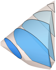
Design a minimum-weight truss that is anchored on one end of the wall and must withstand a load on the other end:
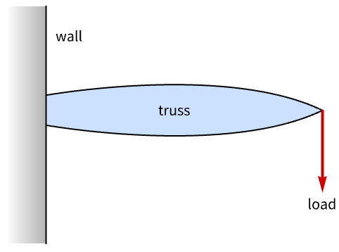
The truss can be modeled using links and nodes. Each node is connected to a neighboring node by a link. Specify the node positions ![]() :
:
nodes = Flatten[Outer[List, {0, 1, 2}, {0, 1, 2}], 1];
nNodes = Length[nodes];
Specify the nodes that are anchored to the wall:
anchorPoints = {{0, 0}, {0, 1}, {0, 2}};Specify the node at which the load is applied:
forcingPoint = {2, 0};Specify the nodes that are connected to each other through a link and compute the length of each link:
links = {...};
linkLengths = Table[EuclideanDistance@@nodes[[ni]], {ni, links}];
nLinks = Length[links];
Visualize the unoptimized truss:
plot = Show[Graphics[GraphicsComplex[...]], Graphics[...]]The links are circular bars. Each link must be formed from one out of a group of bars of cross sections ![]() . Let
. Let ![]() be a decision vector for each link
be a decision vector for each link ![]() , such that if
, such that if ![]() , then bar
, then bar ![]() is selected. For link
is selected. For link ![]() , the area is then defined as
, the area is then defined as ![]() . The objective is to minimize the weight:
. The objective is to minimize the weight:
areas = {20, 30, 40};
objective = linkLengths.s;
The bar selection constraint is:
barSelectionConstraint = Table[Indexed[s, i] == areas.x[i], {i, nLinks}];Only one bar must be selected for each link. The binary constraint is:
binaryConstraint = Table[{Total[x[i]] ≤ 1, 0x[i]1}, {i, nLinks}];Find the indices of the nodes that are not anchored:
anchorIndex = Map[Position[nodes, #][[1, 1]]&, anchorPoints];
freeNodeIndex = Complement[Range[nNodes], anchorIndex];
m = Length[freeNodeIndex];
The stiffness matrix of the system is given by ![]() , where
, where ![]() is the total number of nodes,
is the total number of nodes, ![]() is the number of nodes that are anchored and
is the number of nodes that are anchored and ![]() is the set of all the links. The vector
is the set of all the links. The vector ![]() if
if ![]() ;
; ![]() if
if ![]() , else 0:
, else 0:
bEdge[{i_, j_}] := Module[...];Let ![]() be the force vector for the entire system. At each of the nodes that is not anchored, the force is
be the force vector for the entire system. At each of the nodes that is not anchored, the force is ![]() . The node where force is applied is
. The node where force is applied is ![]() :
:
forceIndex = Position[nodes, forcingPoint][[1, 1]];
forceVector = Flatten[Table[If[s == forceIndex, {0, -1}, {0, 0}],
	{s, freeNodeIndex}]];
Let ![]() be the maximum allowable deflection at any node. Let
be the maximum allowable deflection at any node. Let ![]() be displacement of node
be displacement of node ![]() ; then
; then ![]() is satisfied if
is satisfied if ![]() , where
, where ![]() is the stiffness matrix associated with link
is the stiffness matrix associated with link ![]() :
:
stiffnessMatrices = Sum[...];
stiffnessConstant = With[{γ = 0.1}, {...}];
stiffnessConstraint = Inactive[Plus][stiffnessConstant,
stiffnessMatrices]Underscript[, "SemidefiniteCone"]0;vars = Flatten[{s∈Vectors[nLinks, Reals],
Table[x[i]∈Vectors[Length[areas], Integers], {i, nLinks}]}];Find the optimal structure of the truss:
res = SemidefiniteOptimization[objective, {barSelectionConstraint,
	binaryConstraint, stiffnessConstraint}, vars];
Extract the links that are part of the optimal truss:
optlinkPos = Flatten[Position[s /. res, x_ /; x > 1]]Visualize the optimal truss. The links that are part of the optimal truss are colored-coded based on the rod area being used:
colors = {Blue, Purple, Red};
Row[{Graphics[...], LineLegend[...]}]
Properties & Relations (8)
SemidefiniteOptimization gives the global minimum of the objective function:
res = SemidefiniteOptimization[2Subscript[x, 1] + 3Subscript[x, 2], (| | |
| -- | -- |
| x1 | 1 |
| 1 | x2 |)Underscript[, {"SemidefiniteCone", 2}]0, {Subscript[x, 1], Subscript[x, 2]}]Plot the objective function with the minimum value over the feasible region:
Show[Plot3D[2Subscript[x, 1] + 3Subscript[x, 2], {Subscript[x, 1], Subscript[x, 2]}∈ImplicitRegion[...]], Graphics3D[...]]Minimize gives global exact results for semidefinite problems:
Minimize[{2Subscript[x, 1] + 3Subscript[x, 2], (| | |
| -- | -- |
| x1 | 1 |
| 1 | x2 |)Underscript[, {"SemidefiniteCone", 2}]0}, {Subscript[x, 1], Subscript[x, 2]}]%//NCompare to SemidefiniteOptimization:
SemidefiniteOptimization[2Subscript[x, 1] + 3Subscript[x, 2], (| | |
| -- | -- |
| x1 | 1 |
| 1 | x2 |)Underscript[, {"SemidefiniteCone", 2}]0, {Subscript[x, 1], Subscript[x, 2]}, {"PrimalMinimumValue", "PrimalMinimizerRules"}]NMinimize can be used to get inexact results using global methods:
NMinimize[{2Subscript[x, 1] + 3Subscript[x, 2], (| | |
| -- | -- |
| x1 | 1 |
| 1 | x2 |)Underscript[, {"SemidefiniteCone", 2}]0}, {Subscript[x, 1], Subscript[x, 2]}]FindMinimum can be used to obtain inexact results using local methods:
FindMinimum[{2x + 3y, (| | |
| - | - |
| x | 1 |
| 1 | y |)Underscript[, {"SemidefiniteCone", 2}]0}, {x, y}]ConicOptimization is more general than SemidefiniteOptimization:
ConicOptimization[2Subscript[x, 1] + 3Subscript[x, 2], (| | |
| -- | -- |
| x1 | 1 |
| 1 | x2 |)Underscript[, {"SemidefiniteCone", 2}]0, {Subscript[x, 1], Subscript[x, 2]}]SemidefiniteOptimization[2Subscript[x, 1] + 3Subscript[x, 2], (| | |
| -- | -- |
| x1 | 1 |
| 1 | x2 |)Underscript[, {"SemidefiniteCone", 2}]0, {Subscript[x, 1], Subscript[x, 2]}]SecondOrderConeOptimization is a special case of SemidefiniteOptimization:
SecondOrderConeOptimization[10x + 11y, {x + y ≥ 1, {x, y}∈Disk[]}, {x, y}]SemidefiniteOptimization[10x + 11y, {x + y ≥ 1, {x, y}∈Disk[]}, {x, y}]QuadraticOptimization is a special case of SemidefiniteOptimization:
obj = 2x^2 + 20y^2 + 6x y + 5x;
cons = {-x + y ≥ 2, y ≥ 0};QuadraticOptimization[obj, cons, {x, y}]Use auxiliary variable ![]() and minimize
and minimize ![]() with additional constraint
with additional constraint ![]() :
:
SemidefiniteOptimization[t, {obj ≤ t, cons}, {x, y, t}]LinearOptimization is a special case of SemidefiniteOptimization:
LinearOptimization[10.x + 11.y, {x, y}∈RegularPolygon[4], {x, y}]SemidefiniteOptimization[10.x + 11.y, {x, y}∈RegularPolygon[4], {x, y}]Possible Issues (5)
The constraints at the optimal point are satisfied up to some tolerance:
res = SemidefiniteOptimization[2Subscript[x, 1] + 3Subscript[x, 2], (| | |
| -- | -- |
| x1 | 1 |
| 1 | x2 |)Underscript[, {"SemidefiniteCone", 2}]0, {Subscript[x, 1], Subscript[x, 2]}](| | |
| -- | -- |
| x1 | 1 |
| 1 | x2 |)Underscript[, {"SemidefiniteCone", 2}]0 /. resWith default options, the constraint violation tolerance is 10-8:
Eigenvalues[(|    |    |
| -- | -- |
| x1 | 1  |
| 1  | x2 |) /. res]
The minimum value of an empty set or infeasible problem is defined to be ![]() :
:
SemidefiniteOptimization[x, {x ≤ 0, x ≥ 1}, x, "PrimalMinimumValue"]The minimizer is Indeterminate:
SemidefiniteOptimization[x, {x ≤ 0, x ≥ 1}, x]The minimum value for an unbounded set or unbounded problem is ![]() :
:
SemidefiniteOptimization[-(x + y), x + y ≥ 1, {x, y}, "PrimalMinimumValue"]The minimizer is Indeterminate:
SemidefiniteOptimization[-(x + y), x + y ≥ 1, {x, y}]Dual related solution properties for mixed-integer problems may not be available:
SemidefiniteOptimization[x + y, {x + 2y ≥ 3, x ≥ -2}, {x∈Integers, y∈Integers}, {"DualMaximumValue", "DualMaximizer", "DualityGap"}]Although the constraint matrices can be Hermitian, the variables need to be real:
c = {1, 2};Subscript[a, 0] = (| | |
| ----- | ----- |
| 0 | 1 + I |
| 1 - I | 0 |);Subscript[a, 1] = (| | |
| - | - |
| 1 | 0 |
| 0 | 0 |);Subscript[a, 2] = (| | |
| - | - |
| 0 | 0 |
| 0 | 1 |);SemidefiniteOptimization[c.v, {Subscript[a, 1], Subscript[a, 2]}.vUnderscript[, {"SemidefiniteCone", 2}]-Subscript[a, 0], v∈Vectors[2, Complexes]]Vectors[n] automatically evaluates to Vectors[n,Complexes]:
Vectors[n]For problems with no complex numbers in the specification, the vector variable v ∈Vectors[n] is considered real valued; otherwise, you need to explicitly give the domain as Vectors[n,Reals]:
c = {1, 2};
SemidefiniteOptimization[c.v, {Subscript[a, 1], Subscript[a, 2]}.vUnderscript[, {"SemidefiniteCone", 2}]-Subscript[a, 0], v∈Vectors[2, Reals]]Text
Wolfram Research (2019), SemidefiniteOptimization, Wolfram Language function, https://reference.wolfram.com/language/ref/SemidefiniteOptimization.html (updated 2020).
CMS
Wolfram Language. 2019. "SemidefiniteOptimization." Wolfram Language & System Documentation Center. Wolfram Research. Last Modified 2020. https://reference.wolfram.com/language/ref/SemidefiniteOptimization.html.
APA
Wolfram Language. (2019). SemidefiniteOptimization. Wolfram Language & System Documentation Center. Retrieved from https://reference.wolfram.com/language/ref/SemidefiniteOptimization.html