GaussianOrthogonalMatrixDistribution
GaussianOrthogonalMatrixDistribution[σ,n]
行列次元 {n,n},尺度母数 σ のガウス(Gauss)直交行列分布を表す.
GaussianOrthogonalMatrixDistribution[n]
単位尺度母数を持つガウス直交行列分布を表す.
詳細
- GaussianOrthogonalMatrixDistributionはガウス直交アンサンブル(GOE)としても知られている.
- GaussianOrthogonalMatrixDistributionは,対称行列
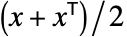 の分布である.ただし,
 は独立同分布に従う行列(その要素はNormalDistribution[0,σ]に従う)を持つ平方行列である.
- 行列
 の確率密度は
 に比例する.
- 尺度母数 σ は任意の正の数でよく,n は任意の正の整数でよい.
- GaussianOrthogonalMatrixDistributionは,MatrixPropertyDistribution,EstimatedDistribution,RandomVariate等の関数とともに使うことができる.
予備知識
- GaussianOrthogonalMatrixDistribution[σ,n]は,ガウス直交アンサンブル(GOE)とも呼ばれるもので,
 実対称行列上の統計分布,具体的には
 を満足する実正方行列
 上の統計分布を表す.ただし,
 は
 の転置を表す.GaussianOrthogonalMatrixDistributionに従って分布する行列
 の確率密度は
 に比例する.さらに,すべての項の集合
 はNormalDistribution[0,σ]に従って一様に分布している実変量の独立集合である.GaussianOrthogonalMatrixDistribution[σ,n]は正の整数 n(次元母数)と正の実数 σ(尺度母数)によってパラメータ化される.「ガウス直交行列分布」という名前ではあるが,この分布に属する行列が直交行列である必要はない.
- 母数が1つの形GaussianOrthogonalMatrixDistribution[n]はGaussianOrthogonalMatrixDistribution[1,n]に等しい.
- ガウス直交行列分布は,ガウスシンプレクティック分布(GaussianSymplecticMatrixDistribution)およびガウスユニタリ分布(GaussianUnitaryMatrixDistribution)と並んで,Eugene Wignerによって原子物理学における揺らぎの研究のツールとして提唱された3つのガウス行列分布の一つである.ガウス直交アンサンブルは,数学的には直交行列による共役のもとで不変であり,物理的には時間反転対称性でハミルトニアンをモデル化する.ガウス直交行列分布のような行列アンサンブルは,ランダム行列理論をはじめとする物理学および数学のさまざま分野の研究において非常に重要である.
- RandomVariateを使って,ガウス直交行列分布から,1つあるいは複数の機械精度あるいは任意精度(後者はWorkingPrecisionオプションを介す)の擬似乱数変量を得ることができる.そのような変量の集合の平均,中央値,分散,モーメント,中心モーメントは,それぞれMean,Median,Variance,Moment,CentralMomentを使って計算することができる.Distributed[A,GaussianOrthogonalMatrixDistribution[σ,n]](より簡単な表記では AGaussianOrthogonalMatrixDistribution[σ,n])を使ってランダム行列 A がガウス直交行列分布に従って分布していると宣言することができる.そのような宣言はMatrixPropertyDistribution等の関数で使うことができる.
- ガウス直交行列分布に従って分布する変量のトレース,固有値,ノルムは,それぞれTr,Eigenvalues,Normを使って計算することができる.そのような変量は,MatrixFunctionやMatrixPowerで調べることもでき,そのような変量の項はMatrixPlotを使ってプロットできる.
- GaussianOrthogonalMatrixDistributionは他の数多くの分布と関係がある.上述の通り,この分布はガウス行列分布のGaussianSymplecticMatrixDistributionおよびGaussianUnitaryMatrixDistributionと定性的に類似している.ガウスアンサンブルの一般化には,いわゆる円行列アンサンブルが含まれるので,GaussianOrthogonalMatrixDistributionはCircularOrthogonalMatrixDistribution,CircularQuaternionMatrixDistribution,CircularRealMatrixDistribution,CircularSymplecticMatrixDistribution,CircularUnitaryMatrixDistributionとも関連している.GaussianOrthogonalMatrixDistributionは,MatrixNormalDistribution,MatrixTDistribution, WishartMatrixDistribution,InverseWishartMatrixDistribution,TracyWidomDistribution,WignerSemicircleDistributionとも関係がある.
例題
すべて開く すべて閉じる例 (4)
RandomVariate[GaussianOrthogonalMatrixDistribution[3]]SymmetricMatrixQ[%]GaussianOrthogonalMatrixDistributionから引かれた行列の項は,ガウス分布を併用し,非相関で,対角から外れる項は対角上の項の半分の分散を持つ:
sample = RandomVariate[MatrixPropertyDistribution[{Indexed[x, {1, 1}], Indexed[x, {2, 2}], Indexed[x, {1, 2}]}, xGaussianOrthogonalMatrixDistribution[2]], 10 ^ 4];DistributionFitTest[sample, MultinormalDistribution[{0, 0, 0}, DiagonalMatrix[{1, 1, 1 / 2}]], "TestConclusion"]MatrixPropertyDistributionを使ってGOE行列の固有値をサンプルする:
RandomVariate[MatrixPropertyDistribution[Eigenvalues[x], xGaussianOrthogonalMatrixDistribution[2000]]]//HistogramMean[GaussianOrthogonalMatrixDistribution[1, 3]]//MatrixFormVariance[GaussianOrthogonalMatrixDistribution[1, 3]]//MatrixFormスコープ (4)
RandomVariate[GaussianOrthogonalMatrixDistribution[2]]MatrixForm /@ RandomVariate[GaussianOrthogonalMatrixDistribution[2], 3]𝒟 = MatrixPropertyDistribution[Det[m], mGaussianOrthogonalMatrixDistribution[4]];NProbability[Abs[det] > 0.1, det𝒟]dist = GaussianOrthogonalMatrixDistribution[2, 3];sample = RandomVariate[dist, 10 ^ 3];edist = EstimatedDistribution[sample, GaussianOrthogonalMatrixDistribution[σ, n]]分布のLogLikelihoodを比較する:
LogLikelihood[#, sample]& /@ {edist, dist}アプリケーション (3)
dist = MatrixPropertyDistribution[{-1, 1}.MinMax[Eigenvalues[x]], xGaussianOrthogonalMatrixDistribution[2]];gaps = Normalize[RandomVariate[dist, 10000], Mean];ヒストグラムをDyson指数  についてのウィグナー(Wigner)推定としても知られる閉形式と比較する:
WignerSurmisePDF[x_, β : 1] := Pi (x / 2) Exp[-Pi (x / 2) ^ 2]Show[Histogram[gaps, {0.1}, PDF], Plot[WignerSurmisePDF[x, 1], {x, 0, 3}]]λ𝒟 = MatrixPropertyDistribution[Eigenvalues[𝓂], 𝓂GaussianOrthogonalMatrixDistribution[2]];RandomSampleを使ってランダムに固有値を置換してアルゴリズム特有の順序を相殺する:
evs = RandomSample /@ RandomVariate[λ𝒟, 10 ^ 5];SmoothHistogram3D[evs]LevelDistribution[n_Integer, β_] := ProbabilityDistribution[(1/(2π)^n / 2)(Underoverscript[∏, j, n](Gamma[1 + (β/2)]/Gamma[1 + (β j/2)]))(Underoverscript[∏, i = 1, n]Underoverscript[∏, j, i - 1]Abs[Subscript[λ, i] - Subscript[λ, j]]^β)Exp[-(1/2)Subsuperscript[∑, i = 1, n]Subscript[λ, i]^2], Array[{Subscript[λ, #], -∞, ∞}&, n, 1, Sequence]]pdf = PDF[LevelDistribution[2, 1], {λ1, λ2}]Show[Histogram3D[evs, {0.5}, PDF, ChartStyle -> Opacity[0.5], PlotRange -> All],
Plot3D[pdf, {λ1, -4, 4}, {λ2, -4, 4}, PlotStyle -> None, MeshStyle -> Thick, PlotRange -> All]]DistributionFitTest[evs, LevelDistribution[2, 1]]inverseTiming[size_] := With[{mat = RandomVariate[GaussianOrthogonalMatrixDistribution[size]]}, RepeatedTiming[Inverse[mat]][[1]]]data = Table[{n, inverseTiming[n]}, {n, {50, 100, 250, 500, 1000, 2000, 3000, 5000}}];ListLogLogPlot[data, Filling -> Axis]特性と関係 (4)
 (
 はGaussianOrthogonalMatrixDistributionからのサンプル)に適用されたMatrixExpは対称かつユニタリである:
MatrixExp[I RandomVariate[GaussianOrthogonalMatrixDistribution[3]]]UnitaryMatrixQ[%] && SymmetricMatrixQ[%]GOE行列の上三角部分の行列要素は独立ガウス確率変数である:
upperElems[n_, symMat_] := Extract[symMat, Join[Table[{k, k}, {k, n}], Subsets[Range[n], {2}]]]MatrixForm[m = RandomVariate[GaussianOrthogonalMatrixDistribution[3]]]upperElems[3, m]IndependenceTestを使って独立性を検証する:
data = RandomVariate[MatrixPropertyDistribution[upperElems[2, x], xGaussianOrthogonalMatrixDistribution[2]], 10 ^ 4];Table[If[i == j, Histogram[data[[All, i]], Automatic, PDF], ListPlot[data[[All, {i, j}]], PlotLabel -> Row[{IndependenceTest[data[[All, i]], data[[All, j]]]}]]], {i, 3}, {j, 3}]//Grid[#, Dividers -> All]&大きいGOE行列のスペクトル密度はWignerSemicircleDistributionに収束する:
n = 300;
eigvs = RandomVariate[MatrixPropertyDistribution[Eigenvalues[x], xGaussianOrthogonalMatrixDistribution[n]], 250];Show[Histogram[(Join@@eigvs) / Sqrt[2n], {0.025}, PDF], Plot[PDF[WignerSemicircleDistribution[1], x], {x, -1, 1}]]大きいGOE行列のスケールされた最大固有値の分布はTracyWidomDistributionに収束する:
n = 300;
Subscript[λ, max] = RandomVariate[MatrixPropertyDistribution[Max[Eigenvalues[x]], xGaussianOrthogonalMatrixDistribution[n]], 10 ^ 3];Show[Histogram[(Subscript[λ, max] - Sqrt[2 n])Sqrt[2] n^1 / 6, {0.3}, PDF], Plot[PDF[TracyWidomDistribution[1], x ], {x, -5, 3}, PlotStyle -> Thick]]テキスト
Wolfram Research (2015), GaussianOrthogonalMatrixDistribution, Wolfram言語関数, https://reference.wolfram.com/language/ref/GaussianOrthogonalMatrixDistribution.html (2017年に更新).
CMS
Wolfram Language. 2015. "GaussianOrthogonalMatrixDistribution." Wolfram Language & System Documentation Center. Wolfram Research. Last Modified 2017. https://reference.wolfram.com/language/ref/GaussianOrthogonalMatrixDistribution.html.
APA
Wolfram Language. (2015). GaussianOrthogonalMatrixDistribution. Wolfram Language & System Documentation Center. Retrieved from https://reference.wolfram.com/language/ref/GaussianOrthogonalMatrixDistribution.html