



ListLogLogPlot
ListLogLogPlot[{y1,y2,…}]
x 座標1, 2, …に対応するとみなされる yiの両対数プロットを作成する.
ListLogLogPlot[{{x1,y1},{x2,y2},…}]
x と y の値の指定したリストの両対数プロットを作成する.
ListLogLogPlot[{data1,data2,…}]
すべての dataiからのデータをプロットする.
ListLogLogPlot[{…,w[datai,…],…}]
記号的ラッパー w で定義された特徴で dataiをプロットする.
詳細とオプション
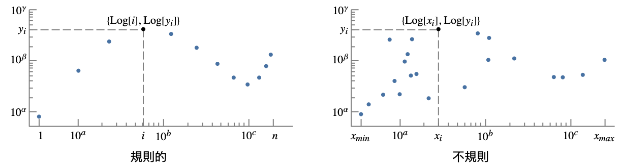
- ListLogLogPlotは事実上Log[xi]とLog[yi]に基づいてプロットするが,目盛はスケールされていない値 xiと yiを示す.
- ListLogLogPlotではベキ乗データが直線に見える.
- データ値 xiおよび yiは次の形式で与えることができる.
-
xi 実数値の数 Quantity[xi,unit] 単位の付いた数量 Around[xi,ei] 不確かさが eiの値 xi Interval[{xmin,xmax}] xminから xmaxまでの値 - 上記の形式ではない値 xiおよび yiは,欠落値とみなされ,表示されない.
- dataiは次の形式と解釈を持つ.
-
<"k1"y1,"k2"y2,…> 値{y1,y2,…} <x1y1,x2y2,…> キーと値のペア {{x1,y1},{x2,y2},…} {y1"lbl1",y2"lbl2",…}, {y1,y2,…}{"lbl1","lbl2",…} ラベル{lbl1,lbl2,…}の付いた値{y1,y2,…} SparseArray 正規配列としての値 TimeSeries, EventSeries 時点と値のペア QuantityArray 大きさ WeightedData 重みのない値 - ListLogLogPlot[Tabular[…]cspec]は,列指定 cspec を使って表形式オブジェクトから値を抽出し,これをプロットする.
- 次は,表形式データのプロットに使用可能な列指定 cspec の形式である.
-
{colx,coly} 列 y と列 x をプロットする {{colx1,coly1},{colx2,coly2},…} 列 y1と列 x1,列 y2と列 x2をプロットする等 coly, {coly} 列 y を一連の値としてプロットする {{coly1},…,{colyi},…} 列 y1, y2, …を一連の値としてプロットする - colxはAutomaticでもよい.その場合は,DataRangeを使って一連の値が生成される.
- ListLogLogPlot[TimeSeries[…]cspec]およびListLogLogPlot[EventSeries[…]cspec]は,成分指定 cspec を用いて時系列または事象系列から値を抽出し,それをプロットする.
- cspec という成分指定の以下の形式は,系列データをプロット には,cspec という成分指定の以下の形式が使用できる.
-
com タイムスタンプに対して成分 com をプロットする {com1,com2,…} 各成分 comi をタイムスタンプに対してプロットする - dataiには,次のラッパー w を使うことができる.
-
Annotation[datai,label] データに注釈を与える Button[datai,action] データがクリックされた際に実行するアクションを定義する Callout[datai,label] コールアウトでデータにラベルを付ける Callout[datai,label,pos] 相対的な位置 pos にコールアウトを置く EventHandler[datai,…] データの一般的なイベントハンドラを定義する Highlighted[fi,effect] 効果を使って fiを動的にハイライトする Highlighted[fi,Placed[effect,pos]] 位置 pos で効果を使って fiを静的にハイライトする Hyperlink[datai,uri] データをハイパーリンクにする Labeled[datai,label] データにラベルを付ける Labeled[datai,label,pos] 相対的な位置 pos にラベルを置く Legended[datai,label] データを凡例で識別する PopupWindow[datai,cont] データにポップアップウィンドウを付ける StatusArea[datai,label] マウスが来たときにステータスエリアに表示する Style[datai,styles] 指定したスタイルを使ってデータを示す Tooltip[datai,label] データにツールチップを付ける Tooltip[datai] データの値をツールチップとして使う - ラッパー w は複数のレベルで適用することができる.
-
{…,w[yi],…} データの値 yiを囲む {…,w[{xi,yi}],…} 点{xi,yi}を囲む w[datai] データを囲む w[{data1,…}] dataiの集合を囲む w1[w2[…]] ネストしたラッパーを使う - Callout,Labeled,Placedには次の位置 pos が使える.
-
Automatic 自動的に置かれたラベル Above, Below, Before, After データの周りの位置 x 位置 x のデータの近く Scaled[s] データに沿ってスケールされた位置 s {s,Above},{s,Below},… データに沿った位置 s の相対的な位置 {pos,epos} データと相対的な位置 pos に置かれたラベル中の epos - ListLogLogPlotには,Graphicsと同じオプションに以下の追加・修正を加えたものが使える. [全オプションのリスト]
-
AspectRatio 1/GoldenRatio 縦横比 Axes True 軸を描くかどうか DataRange Automatic データとして推測する x の値の範囲 IntervalMarkers Automatic 不確かさをどのように描画するか IntervalMarkersStyle Automatic 不確かな要素のスタイル Filling None 各点の幹をどのように塗り潰すか FillingStyle Automatic 塗潰しに使うスタイル Joined Automatic 点を繋ぐかどうか LabelingFunction Automatic どのうように点にラベルを付けるか LabelingSize Automatic コールアウトとラベルの最大サイズ LabelingTarget Automatic 自動のラベル配置の決定方法 PerformanceGoal $PerformanceGoal パフォーマンスのどの面について最適化するか PlotFit None 曲線を点にフィットする方法 PlotFitElements Automatic プロットに表示するフィット要素 PlotHighlighting Automatic データのハイライト効果 PlotInteractivity $PlotInteractivity インタラクティブ要素を許可するかどうか PlotLabel None プロットの全体的なラベル PlotLabels None データのラベル PlotLayout "Overlaid" データ配置の決め方 PlotLegends None データの凡例 PlotMarkers None 各点を表すためのマーカー PlotRange Automatic 含める値の範囲 PlotRangeClipping True プロット範囲で切り取るかどうか PlotStyle Automatic 点のスタイルを決定するグラフィックス指示子 PlotTheme $PlotTheme 全体的なプロットのテーマ ScalingFunctions None 個々の座標のスケール方法 TargetUnits Automatic プロット内に表示する単位 - DataRangeは,値{y1,…,yn}をどのように{{x1,y1},…,{xn,yn}}と解釈するかを決定する.次は使用可能な設定である.
-
Automatic,All 1から n まで一様に {xmin,xmax} xminから xmaxまで一様に - 一般に,ペア{{x1,y1},{x2,y2},…}のリストは点のリストと解釈されるが,設定DataRangeAllはそれを複数の datai {{y11,y12},{y21,y23},…}として解釈するように強制する.
- LabelingFunction->f は,各点に f[value,index,lbls]で与えられるラベルを付けるように指定する.value は点に関連付けられた値,index は data 中の位置,lbls は関連するラベルのリストである.
- 次は,単一のプロットパネルで複数の曲線を表示する際のPlotLayoutの可能な設定である.
-
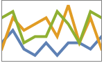
"Overlaid" すべてのデータを重ねて表示する 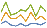
"Stacked" データを積み重ねる 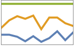
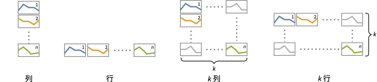
"Percentile" データを重ねて正規化する - 次は,複数のプロットパネルで単一の曲線を表示する際のPlotLayoutの可能な設定である.
-
"Column" パネルの列で別々の曲線を使う "Row" パネルの行で別々の曲線を使う {"Column",k},{"Row",k} k 列(行)使う {"Column",UpTo[k]},{"Row",UpTo[k]} 最大で k 列(行)使う - 次は,PlotLegendsによく使われる設定である.
-
None 凡例は使わない Automatic 凡例を自動的に決定する {lbl1,lbl2,…} lbl1, lbl2, …を凡例ラベルとして使う Placed[lspec,…] 凡例の置き方を指定する - PlotStylesty は,各曲線に使用するスタイルを指定する.可能な設定には次が含まれる.
-
{sty1,sty2,…} データ集合のためのスタイルの列 <"key"val,…> データの異なるレベルに対するスタイル要素 - 受け入れられるキーは次の通りである.
-
"Base" すべての dataiに対する全体的なスタイル "Lists" dataiごとのスタイル styiのリスト - ColorData["DefaultPlotColors"]は,PlotStyleで使われるデフォルトの色のシーケンスを与える.
- 次は,ScalingFunctionsの可能な設定である.
-
sy y 軸をスケールする {sx,sy} x 軸と y 軸をスケールする - 次は,よく使われる組込みのスケーリング関数 s である.
-
"Reverse" 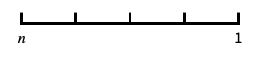
座標の向きを逆にする "Infinite" 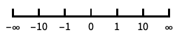
無限スケール - x 軸と y 軸についてのスケールはデフォルトの対数スケールの後で適用される.
- 次は,HighlightedとPlotHighlightingに使用可能なハイライト効果である.
-
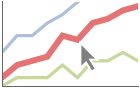
style 指定された曲線をハイライトする 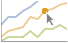
"Ball" 曲線上の指定された点をハイライトしてラベルを付ける 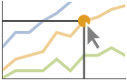
"Dropline" 曲線上の指定された点を軸までのドロップラインでハイライトしてラベルを付ける 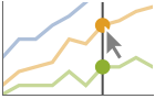
"XSlice" 垂直スライスに沿ったすべての点をハイライトしてラベルを付ける 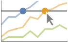
"YSlice" 水平スライスに沿ったすべての点をハイライトしてラベルを付ける 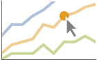
Placed[effect,pos] 指定の位置 pos を静的にハイライトする - ハイライトの位置指定 pos には次がある.
-
x, {x} {x,y}における効果.y は自動的に選択される {x,y} {x,y}における効果 {pos1,pos2,…} 複数の位置 posi
全オプションのリスト
例題
すべて開く すべて閉じる例 (5)
ListLogLogPlot[Range[20] ^ 3]ListLogLogPlot[Range[20] ^ 3, Joined -> True]

ListLogLogPlot[Table[{n Log[n], Prime[n]}, {n, 20}]]ListLogLogPlot[{Range[20], Sqrt[Range[20]], Log[Range[20]]}, Joined -> True, PlotLegends -> {"one", "two", "three"}]{data1, data2, data3} = Transpose[Table[{n, 2 ^ n, Fibonacci[n]}, {n, 10}]];ListLogLogPlot[{data1, data2, data3}, Joined -> True, PlotLabels -> {n, 2 ^ n, Fibonacci[n]}]ListLogLogPlot[Range[20] ^ 3, Filling -> Bottom]ListLogLogPlot[Range[20] ^ 3, Filling -> Bottom, Joined -> True]スコープ (56)
一般的なデータ (10)
 値からなる規則的なデータについては,
 のデータ範囲は整数値であるとみなされる:
ListLogLogPlot[Range[40]]DataRangeを使って明示的な  のデータ範囲を与える:
ListLogLogPlot[Range[40], DataRange -> {0, 1}]ListLogLogPlot[{Sqrt[Range[40]], Log[Range[40, 80]]}] と
 の値のペアからなる不規則データについては,
 のデータ範囲はデータから推測される:
data = Last[Reap[NIntegrate[1 / x ^ 2, {x, 0.1, 2}, EvaluationMonitor :> Sow[{x, 1 / x ^ 2}]]]];ListLogLogPlot[data]data1 = Table[{x, x ^ 3}, {x, RandomReal[20, 50]}];
data2 = Table[{x, x ^ 5}, {x, RandomReal[20, 250]}];ListLogLogPlot[{data1, data2}]DataRangeを使って規則的あるいは不規則な複数のデータ集合を同じ  範囲にマップしてプロットする:
data1 = Table[x ^ 2, {x, 1, 10, 0.5}];
data2 = Table[{x, x ^ 5}, {x, RandomReal[10, 250]}];ListLogLogPlot[{data1, data2}, DataRange -> {1, 10}]ListLogLogPlot[{1, 2, 3, 1 + I, 4, 5, 6, None, 7, 8, 9, Missing["NotAvailable"], 10, 11, 12}, Joined -> True, Mesh -> All]ListLogLogPlot[Sin[Range[0, 3Pi, 0.1]], Joined -> True, Mesh -> All]MaxPlotPointsを使って使用する点の数を制限する:
Table[ListLogLogPlot[Table[{n, (Sin[3n] + 1)Gamma[n]}, {n, 0, 10, 0.01}], MaxPlotPoints -> mp, Joined -> True, Mesh -> All], {mp, {Infinity, 50, 30}}]PlotRangeは自動的に選択される:
{ListLogLogPlot[{0, 1, 2, 3, 500, 5, 6, 7}, Joined -> True], ListLogLogPlot[{0, 1, 2, 3, 500, 5, 6, 7}, Joined -> True, PlotRange -> All]}PlotRangeを使って関心領域に焦点を当てる:
{ListLogLogPlot[Table[{x, Exp[x] / Abs[x - 2]}, {x, 0, 5, 0.05}]], ListLogLogPlot[Table[{x, Exp[x] / Abs[x - 2]}, {x, 0, 5, 0.05}], PlotRange -> {10, 100}]}//QuietScalingFunctionsを使って y 軸の向きを逆にする:
ListLogLogPlot[Table[Power[E, x], {x, 0, 50}], ScalingFunctions -> "Reverse"]ListLogLogPlot[Table[Power[E, x], {x, 0, 50}], ScalingFunctions -> {"Reverse", "Reverse"}]特殊データ (9)
Quantityを使ってデータに単位を加える:
ListLogLogPlot[Quantity[Sqrt[Range[10]], "Meters"], AxesLabel -> Automatic]

data = EntityValue[EntityClass["Element", All], {"AtomicMass", "MeltingPoint"}];ListLogLogPlot[data, AxesLabel -> Automatic]QuantityArray内のデータをプロットする:
data = QuantityArray[EntityValue[EntityClass["Element", All], {"AtomicMass", "MeltingPoint"}]]ListLogLogPlot[data, AxesLabel -> Automatic]TargetUnitsを使って使用する単位を指定する:
ListLogLogPlot[data, TargetUnits -> {Automatic, "Kelvin"}, AxesLabel -> Automatic]ListLogLogPlot[Table[Around[RandomReal[100], RandomReal[1]], 20]]ListLogLogPlot[Table[Interval[RandomReal[{1, 100}, 2]], 20]]ListLogLogPlot[{2 -> "a", 3 -> "b", 5 -> "c", 7 -> "d", 11 -> "e", 13 -> "f", 17 -> "g"}]ListLogLogPlot[{2, 3, 5, 7, 11, 13, 17} -> {"a", "b", "c", "d", "e", "f", "g"}]ListLogLogPlot[{2, 3, 5, 7, 11, 13, 17} -> {"a", "b", "c", "d", "e", "f", "g"}, LabelingFunction -> Above]Association内の数値は  座標として使われる:
ListLogLogPlot[<|"a" -> 2, "b" -> 3, "c" -> 5, "d" -> 7, "e" -> 11, "f" -> 13|>]Association内の数値によるキーと値は  座標と
 座標として使われる:
ListLogLogPlot[<|2 -> 1, 3 -> 2, 5 -> 3, 7 -> 4, 11 -> 5, 13 -> 6|>]TimeSeriesを直接プロットする:
data = CountryData["UnitedStates", {{"Population"}, {1988, 2013}}]ListLogLogPlot[data, AxesLabel -> Automatic]SparseArray内のデータをプロットする:
ListLogLogPlot[SparseArray[Table[Prime[i] -> 1, {i, 25}]]]WeightedData内の重みは無視される:
ListLogLogPlot[WeightedData[{2, 3, 5, 7, 11, 13, 17, 19, 23, 29}, {1, 2, 3, 4, 5, 6, 7, 8, 9, 10}]]表形式データ (3)
tab = EntityValue["Country", {"Name", "Continent", "Population", "GDP"}, "Tabular"]ListLogLogPlot[tab -> {"Population", "GDP"}]GDPデータが大陸ごとに分割されるようにデータをピボットする:
pivot = PivotToColumns[tab, "Continent" -> "GDP"]ListLogLogPlot[pivot -> {{"Population", EntityClass["Country", "NorthAmerica"]}, {"Population", EntityClass["Country", "SouthAmerica"]}}, PlotLegends -> {"North America", "South America"}, Rule[...]]TimeSeriesまたはEventSeriesのすべてのデータをプロットする:
ListLogLogPlot[TimeSeries[TimeEventSeries`TimestampData[Association["UniformlySpacedQ" -> False,
   "Timestamps" -> TabularColumn[Association[
      "Data" -> {7, {{NumericArray[{-248, 118, 298, 638, 865, 1006, 1216}, "Integer32"], {},
          None}}, None},  ...   "Data" -> {{32, 62, 112, 167, 179, 209, 214}, {}, None}, "ElementType" -> "Integer64"]],
         TabularColumn[Association["Data" -> {{30, 49, 81, 125, 142, 174, 177}, {}, None},
"ElementType" -> "Integer64"]]}}]]]], Association[]]]TimeSeriesまたはEventSeriesの特定の成分をプロットする:
trees = TimeSeries[TimeEventSeries`TimestampData[Association["UniformlySpacedQ" -> False,
   "Timestamps" -> TabularColumn[Association[
      "Data" -> {7, {{NumericArray[{-248, 118, 298, 638, 865, 1006, 1216}, "Integer32"], {},
          None}}, None},  ...   "Data" -> {{32, 62, 112, 167, 179, 209, 214}, {}, None}, "ElementType" -> "Integer64"]],
         TabularColumn[Association["Data" -> {{30, 49, 81, 125, 142, 174, 177}, {}, None},
"ElementType" -> "Integer64"]]}}]]]], Association[]];ListLogLogPlot[trees -> "tree 1"]ListLogLogPlot[trees -> {"tree 1", "tree 2"}]データのラッパー (6)
個々のデータ,データ集合,データ集合の集合にラッパーを使う:
{ListLogLogPlot[{{1, Style[2, Red], 3}, {4, 5, 6}}, PlotStyle -> PointSize[0.05]], ListLogLogPlot[{Style[{1, 2, 3}, Green], {4, 5, 6}}, PlotStyle -> PointSize[0.05]], ListLogLogPlot[Style[{{1, 2, 3}, {4, 5, 6}}, Blue], PlotStyle -> PointSize[0.05]]}{ListLogLogPlot[{{1, Style[2, Red], 3}, {4, 5, 6}}, PlotStyle -> PointSize[0.05]], ListLogLogPlot[{Style[{1, Style[2, Red], 3}, Green], {4, 5, 6}}, PlotStyle -> PointSize[0.05]], ListLogLogPlot[Style[{Style[{1, Style[2, Red], 3}, Green], {4, 5, 6}}, Blue], PlotStyle -> PointSize[0.05]]}ListLogLogPlot[Tooltip[Prime[Range[100]]]]ListLogLogPlot[Tooltip[Prime[Range[100]], "primes"]]ListLogLogPlot[Table[Labeled[RandomReal[1, 2], i], {i, 20}], PlotStyle -> PointSize[Medium], ImageSize -> 300]PopupWindowを使って追加的なドリルダウン情報を加える:
ListLogLogPlot[{1, PopupWindow[2, DateListPlot[FinancialData["IBM", "Jan. 1, 2004"]]], 3}, PlotStyle -> PointSize[0.05]]Buttonを使って任意のアクションを引き起こすことができる:
ListLogLogPlot[{1, Button[2, Speak[2]], 3}, PlotStyle -> PointSize[0.05]]ラベルと凡例 (16)
ListLogLogPlot[Table[Labeled[RandomReal[1, 2], i], {i, 20}]]Table[ListLogLogPlot[Table[Labeled[RandomReal[1, 2], i, p], {i, 5}], PlotLabel -> p], {p, {Above, Below, Before, After}}]Labeledでデータにラベルを付ける:
data = Table[Table[{x, f}, {x, 0, 2Pi, 0.1}], {f, {Exp[x], Log[2x]}}];ListLogLogPlot[MapThread[Labeled[#1, #2]&, {data, {Exp[x], Log[2x]}}]]PlotLabelsでデータにラベルを付ける:
data = Table[Table[{x, f}, {x, 0, 2Pi, 0.1}], {f, {Exp[x], Exp[x + 2]}}];ListLogLogPlot[data, PlotLabels -> {Exp[x], Exp[x + 2]}]
ListLogLogPlot[Labeled[Table[{x, Exp[x]}, {x, .1, 2Pi, 0.1}], "exp(x)", 3]]ListLogLogPlot[Labeled[Table[{x, Log[x]}, {x, 1.1, 2Pi, 0.1}], "log(x)", Scaled[0.25]]]ListLogLogPlot[Labeled[Table[{x, Log[x]}, {x, 1.1, 2Pi, 0.1}], Log[x], {Scaled[0.25], Above}]]Calloutでデータに自動的にラベルを付ける:
ListLogLogPlot[{Callout[Table[PartitionsQ[n], {n, 18}], PartitionsQ[n]], Callout[Table[n, {n, 18}], n]}]ListLogLogPlot[Callout[Table[n ^ Sin[n], {n, 1, 10, 0.25}], "label", Above]]ListLogLogPlot[Callout[Table[n ^ Sin[n], {n, 1, 10, 0.25}], "label", 5]]LabelingFunctionでラベルの名前を指定する:
ListLogLogPlot[Prime[Range[10]], LabelingFunction -> (#1 &)]data = Table[Labeled[Prime[i], RandomWord[]], {i, 10}];ListLogLogPlot[data, LabelingSize -> 30]ListLogLogPlot[data, LabelingSize -> Full]密な点集合については,デフォルトで,ラベルの中にツールチップに変換されるものがあるかもしれない:
data = Table[Callout[RandomReal[1, 2], i], {i, 100}];ListLogLogPlot[data]プロットサイズを大きくすると,より多くのラベルが表示される:
ListLogLogPlot[data, ImageSize -> 400]data = Table[Table[{x, f}, {x, 0, 2Pi, 0.1}], {f, {Log[x], Exp[2x]}}];ListLogLogPlot[data, PlotLegends -> {Log[x], Exp[2x]}]Legendedを使って特定のデータ集合に凡例を付ける:
upper = RandomReal[{1.5, 2}, 50];
lower = RandomReal[0.5, 50];ListLogLogPlot[{lower, Legended[Mean[{lower, upper}], "average"], upper}]Placedを使って凡例の位置を変える:
ListLogLogPlot[{lower, Legended[Mean[{lower, upper}], Placed["average", Below]], upper}]ListLogLogPlot[<|"fibonacci" -> Fibonacci[Range[10]], "primes" -> Prime[Range[10]]|>, PlotLabels -> Automatic, PlotLegends -> None]プロットには,通常,マウスオーバーの際に座標を示すインタラクティブなコールアウトが付いている:
ListLogLogPlot[{IconizedObject[«Fibonacci»], IconizedObject[«Primes»]}]特定のラッパーあるいはツールチップのようなインタラクションを含めてインタラクティブ機能をオフにする:
ListLogLogPlot[Callout[IconizedObject[«Fibonacci»], "hello", 10]]{ListLogLogPlot[{IconizedObject[«Fibonacci»], IconizedObject[«Primes»]}, PlotHighlighting -> "Dropline"], ListLogLogPlot[{IconizedObject[«Fibonacci»], IconizedObject[«Primes»]}, PlotHighlighting -> "XSlice"]}Highlightedを使ってプロット上の特定の点を強調する:
ListLogLogPlot[Highlighted[IconizedObject[«Fibonacci»], Placed["Ball", 7]]]ListLogLogPlot[Highlighted[IconizedObject[«Fibonacci»], Placed["Ball", {{3}, {8}}]]]プレゼンテーション (12)
data = Table[Table[{x, f}, {x, 0, 10, 0.1}], {f, {Exp[x], Gamma[x]}}];ListLogLogPlot[data]data = Table[Table[{x, f}, {x, 0, 10, 0.1}], {f, {Exp[x], Gamma[x]}}];ListLogLogPlot[data, PlotStyle -> {Blue, Red}]data = Table[Table[{x, f}, {x, 0, 10, 0.1}], {f, {Exp[x], Gamma[x]}}];ListLogLogPlot[data, PlotLegends -> {Exp[x], Gamma[x]}]ListLogLogPlot[Table[{k, Binomial[30, k]}, {k, 0, 31}], AxesLabel -> {k, None}, PlotLabel -> Binomial[30, k], PlotStyle -> Directive[PointSize[Medium], Purple]]データにインタラクティブな Tooltipを与える:
ListLogLogPlot[Table[Tooltip[x, If[PrimeQ[x], Row[{"prime: ", x}], x]], {x, 1, 25}], PlotStyle -> Directive[PointSize[Medium], Orange]]data = Table[Tooltip[Table[{x, f}, {x, 0, 10, 0.1}], TraditionalForm[f]], {f, {Exp[x], Gamma[x]}}];ListLogLogPlot[data, Joined -> True, PlotStyle -> Thick]data = Table[Table[{x, f}, {x, 0, 10, 0.1}], {f, {Exp[x], Gamma[x]}}];ListLogLogPlot[data, Filling -> {1 -> {2}}, FillingStyle -> {Red, Blue}]ListLogLogPlot[{{1, 2, 3, 5, 8}, {2, 3, 6, 9, 10}, {4, 5, 10, 14, 16}}, PlotMarkers -> Automatic]ListLogLogPlot[{{1, 2, 3, 5, 8}, {2, 3, 6, 9, 10}, {4, 5, 10, 14, 16}}, PlotMarkers -> {"1", "2", "3"}]Joinedを使ってデータ集合を線で繋ぐ:
ListLogLogPlot[{1, 2, 4, 7, 3, 5, 8, 10, 9}, Joined -> True, PlotStyle -> Orange]InterpolationOrderを使って繋いだデータを滑らかにする:
Table[ListLogLogPlot[{2, 4, 16, 128, 8, 32, 256, 1024, 512}, Joined -> True, InterpolationOrder -> io, PlotStyle -> Dashed], {io, {0, 1, 2, 3}}]ListLogLogPlot[Table[Table[{x, f}, {x, 0, 10, 0.1}], {f, {Exp[x], Gamma[x]}}], PlotTheme -> "Detailed"]ListLogLogPlot[Table[Table[{x, f}, {x, 0, 10, 0.1}], {f, {Exp[x], Gamma[x]}}], PlotTheme -> "Marketing"]data = {{10, 9, 4, 3, 5, 3, 5, 5, 2, 6}, {2, 10, 5, 6, 9, 4, 9, 3, 7, 2}, {7, 8, 3, 4, 4, 2, 6, 3, 8, 7}};ListLogLogPlot[data, PlotLayout -> "Stacked", Joined -> True]ListLogLogPlot[data, PlotLayout -> "Percentile", Joined -> True]オプション (143)
ClippingStyle (6)
ClippingStyleはJoinedのデータ集合にのみ適用される:
data = Table[{x, Tan[x]}, {x, -2 Pi, 2 Pi, .1}];//Quiet{ListLogLogPlot[data, ClippingStyle -> Red, PlotRange -> {{.1, 3}, {.01, 1}}], ListLogLogPlot[data, ClippingStyle -> Red, Joined -> True, PlotRange -> {{.1, 3}, {.01, 1}}]}data = Table[{x, Tan[x]}, {x, -2 Pi, 2 Pi, .1}];//QuietListLogLogPlot[data, ClippingStyle -> None, Joined -> True, PlotRange -> {{.01, 3}, All}]data = Table[{x, Tan[x]}, {x, -2 Pi, 2 Pi, .1}];//QuietListLogLogPlot[data, ClippingStyle -> Automatic, PlotStyle -> Thick, Joined -> True, PlotRange -> {All, {.5, 1}}]data = Table[{x, Tan[x]}, {x, -2 Pi, 2 Pi, .1}];//QuietListLogLogPlot[data, ClippingStyle -> Red, Joined -> True, PlotRange -> {{1.2, 1.5}, {.1, 5}}]data = Table[{x, Tan[x]}, {x, -2 Pi, 5Pi, .1}];//QuietListLogLogPlot[data, ClippingStyle -> {Red, Thick}, Joined -> True, PlotRange -> {All, {.1, 1}}, AxesOrigin -> {.1, .3}]data = Table[{x, Tan[x]}, {x, -2 Pi, 5Pi, .1}];//QuietListLogLogPlot[data, ClippingStyle -> Directive[Red, Thick], Joined -> True, PlotRange -> {All, {.1, 1}}, AxesOrigin -> {.1, .3}]ColorFunction (6)
ColorFunctionはJoinedのデータ集合のみに適用される:
{ListLogLogPlot[Table[{x, Gamma[x]}, {x, 1, 7, 0.1}], ColorFunction -> "Rainbow"], ListLogLogPlot[Table[{x, Gamma[x]}, {x, 1, 7, 0.1}], ColorFunction -> "Rainbow", Joined -> True]}

Table[ListLogLogPlot[Table[{x, Gamma[x]}, {x, 1, 7, 0.1}], Joined -> True, ColorFunction -> Function[{x, y}, Evaluate[f]], PlotLabel -> f, PlotStyle -> Thick], {f, {Hue[x], Hue[y]}}]ListLogLogPlot[Table[{x, Gamma[x]}, {x, 1, 7, 0.1}], Joined -> True, ColorFunction -> "DarkRainbow"]ListLogLogPlot[Table[{x, Gamma[x]}, {x, 1, 7, 0.1}], Joined -> True, ColorFunction -> Function[{x, y}, Hue[x]], Filling -> Axis]ColorFunctionは,曲線の彩色では,PlotStyleより優先順位が高い:
ListLogLogPlot[Table[{x, Gamma[x]}, {x, 1, 7, 0.1}], Joined -> True, ColorFunction -> "DarkRainbow", PlotStyle -> Directive[Red, Thick]]MeshShadingでAutomaticを使ってColorFunctionを使う:
ListLogLogPlot[Table[{x, Gamma[x]}, {x, 1, 7, 0.1}], Joined -> True, ColorFunction -> "Rainbow", PlotStyle -> Directive[Red, Thick], Mesh -> 10, MeshShading -> {Automatic, StandardGray}, MeshStyle -> None]ColorFunctionScaling (3)
ColorFunctionScalingはJoinedのデータ集合にのみ適用される:
{ListLogLogPlot[Range[10], ColorFunction -> "Rainbow", ColorFunctionScaling -> True], ListLogLogPlot[Range[10], Joined -> True, ColorFunction -> "Rainbow", ColorFunctionScaling -> True]}左側には引数のないスケーリングを,右側には自動スケーリングを使う:
Table[ListLogLogPlot[Table[Gamma[x], {x, 1, 7}], PlotStyle -> Thick, ColorFunction -> Function[{x, y}, Hue[y]], ColorFunctionScaling -> cf, Joined -> True], {cf, {False, True}}]Table[ListLogLogPlot[Table[Exp[t], {t, 0, 2 ^ i, 0.1}], Joined -> True, PlotStyle -> Thick, ColorFunction -> Function[{x, y}, Hue[y]]], {i, {0, 2, 4}}]ListLogLogPlot[Table[Gamma[x], {x, 1, 7, 0.1}], Joined -> True, ColorFunction -> Function[{x, y}, Hue[Log[10, y]]], PlotStyle -> Thick, ColorFunctionScaling -> False]DataRange (5)
ListLogLogPlot[Table[Exp[x], {x, 0, 3, 0.1}]]ListLogLogPlot[Table[Exp[x], {x, 0, 3, 0.1}], DataRange -> {0, 3}]ListLogLogPlot[{Factorial[Range[30]], Exp[Range[10, 50]]}, DataRange -> {1, 5}]

ListLogLogPlot[Table[{i + 10, i!}, {i, 25}], AxesOrigin -> {1, 0}] 値がデータの一部なので,DataRangeを指定してもこの場合は影響がない:
ListLogLogPlot[Table[{i + 10, i!}, {i, 25}], AxesOrigin -> {1, 0}, DataRange -> {1, 10}]ListLogLogPlot[{{1, 4}, {2, 2}, {3, 3}}, DataRange -> All, AxesOrigin -> {0, 0}, Joined -> True]Filling (8)
Table[ListLogLogPlot[Table[Prime[n], {n, 30}], Filling -> c], {c, {Top, Bottom, Axis, Prime[15]}}]ListLogLogPlot[{Range[20], Table[Prime[n], {n, 20}]}, Filling -> {1 -> {2}}]ListLogLogPlot[{Range[20], Table[Prime[n], {n, 20}]}, Filling -> {1 -> {{2}, Directive[Orange, Dashed]}}]データ集合1とデータ集合2の間を塗り潰す.1が2より小さい場合は赤を,それ以外の場合は青を使う:
data1 = Factorial[Range[30]];
data2 = Exp[Range[30] + 15];ListLogLogPlot[{data1, data2}, Filling -> {1 -> {{2}, {Red, Blue}}}]data = Last[Reap[Plot[Abs[Tan[x]], {x, 0, 10}, EvaluationMonitor :> Sow[{x, Abs[Tan[x]]}]]]];ListLogLogPlot[data, Filling -> Axis]data1 = First@Last[Reap[Plot[Abs[Tan[x]], {x, 0, 2Pi}, EvaluationMonitor :> Sow[{x, Abs[Tan[x]]}]]]];
data2 = First@Last[Reap[Plot[Abs[Cot[x]], {x, 0, 2Pi}, EvaluationMonitor :> Sow[{x, Abs[Cot[x]]}]]]];ListLogLogPlot[{Sort@data1, Sort@data2}, Filling -> {1 -> {2}}]Joinedのデータ集合は単色で塗り潰される:
ListLogLogPlot[{Range[20], Table[{n + 1 / 2, Prime[n]}, {n, 20}]}, Filling -> {1 -> {2}}, Joined -> True]塗潰しのタイプは最初の集合が繋がれているかどうかに依存する:
Table[ListLogLogPlot[{Range[20], Range[20] / 2}, Joined -> {True, False}, Filling -> f, PlotLabel -> f], {f, {1 -> {2}, 2 -> {1}}}]FillingStyle (4)
ListLogLogPlot[Table[Prime[n], {n, 20}], Filling -> Axis, FillingStyle -> Blue]ListLogLogPlot[Table[Prime[n], {n, 20}], Filling -> Axis, FillingStyle -> Directive[Magenta, Dashed]]
ListLogLogPlot[Table[{x, Gamma[x]}, {x, 0, 10, 0.2}], Filling -> 100, FillingStyle -> {Red, Blue}]ListLogLogPlot[Table[Prime[n], {n, 20}], Filling -> Axis, Joined -> True]InterpolationOrder (5)
Joinedで作られた線は補間することができる:
ListLogLogPlot[{{1, 4, 2, 3, 10, 8, 2}}, Joined -> True, InterpolationOrder -> 2]ListLogLogPlot[{{1, 4, 2, 3, 10, 8, 2}}, Joined -> True, InterpolationOrder -> None, Mesh -> Full]ListLogLogPlot[{{1, 4, 2, 3, 10, 8, 2}}, Joined -> True, InterpolationOrder -> 0, Mesh -> Full]ListLogLogPlot[{{1, 4, 2, 3, 10, 8, 2}}, Joined -> True, InterpolationOrder -> 3, Mesh -> Full]Table[ListLogLogPlot[{{1, 4, 2, 3, 10, 8, 2}}, Joined -> True, InterpolationOrder -> i, Mesh -> Full, PlotLabel -> i], {i, 0, 5}]IntervalMarkers (3)
ListLogLogPlot[Table[Around[RandomReal[{50, 100}], 10], 10]]ListLogLogPlot[Table[Around[RandomReal[{50, 100}], 10], 10], IntervalMarkers -> "Bars"]ListLogLogPlot[Table[Around[RandomReal[{0.5, 1}], .1], 10], IntervalMarkers -> "Bands", Joined -> True]IntervalMarkersStyle (2)
ListLogLogPlot[{Table[Around[RandomReal[{50, 100}], 10], 10], Table[Around[RandomReal[{150, 200}], 10], 10]}, PlotMarkers -> Automatic]ListLogLogPlot[{Table[Around[RandomReal[{50, 100}], 10], 10], Table[Around[RandomReal[{150, 200}], 10], 10]}, IntervalMarkersStyle -> Gray, PlotMarkers -> Automatic]Joined (6)
ListLogLogPlot[Table[Prime[n], {n, 20}], Joined -> True]ListLogLogPlot[{Range[20], Table[Prime[n], {n, 20}]}, Joined -> {True, False}]ListLogLogPlot[Table[Prime[n], {n, 20}], Joined -> True, Mesh -> All]TimeSeriesは連続した線として表示される:
ListLogLogPlot[TimeSeries[TimeEventSeries`TimestampData[Association["UniformlySpacedQ" -> False,
   "Timestamps" -> TabularColumn[Association[
      "Data" -> {12, {{NumericArray[{20089, 20120, 20148, 20179, 20209, 20240, 20270, 20301, 20332,
           20362,  ...       146, 166}, {}, None}, "ElementType" -> "Integer64"]],
         TabularColumn[Association["Data" -> {{204, 188, 235, 227, 234, 264, 302, 293, 259, 229,
203, 229}, {}, None}, "ElementType" -> "Integer64"]]}}]]]], Association[]]]EventSeriesは離散点として表示される:
ListLogLogPlot[EventSeries[TimeEventSeries`TimestampData[Association["UniformlySpacedQ" -> False,
   "Timestamps" -> TabularColumn[Association[
      "Data" -> {12, {{NumericArray[{20089, 20120, 20148, 20179, 20209, 20240, 20270, 20301, 20332,
           20362, ...       146, 166}, {}, None}, "ElementType" -> "Integer64"]],
         TabularColumn[Association["Data" -> {{204, 188, 235, 227, 234, 264, 302, 293, 259, 229,
203, 229}, {}, None}, "ElementType" -> "Integer64"]]}}]]]], Association[]]]Table[ListLogLogPlot[{Range[20], Range[20] / 2}, Joined -> {True, False}, Filling -> f, PlotLabel -> f], {f, {1 -> {2}, 2 -> {1}}}]LabelingFunction (6)
ListLogLogPlot[{1, 1, 2, 3, 5, 8} -> {"a", "b", "c", "d", "e", "f"}]LabelingFunction->Noneを使ってラベルが付けられないようにする:
ListLogLogPlot[{1, 1, 2, 3, 5, 8} -> {"a", "b", "c", "d", "e", "f"}, LabelingFunction -> None]ListLogLogPlot[{1, 1, 2, 3, 5, 8} -> {"a", "b", "c", "d", "e", "f"}, LabelingFunction -> Above]ListLogLogPlot[{1, 1, 2, 3, 5, 8} -> {"a", "b", "c", "d", "e", "f"}, LabelingFunction -> Tooltip]ListLogLogPlot[{1, 1, 2, 3, 5, 8} -> {"a", "b", "c", "d", "e", "f"}, LabelingFunction -> Callout[Automatic, Automatic]]ListLogLogPlot[{1, 1, 2, 3, 5, 8} -> {"a", "b", "c", "d", "e", "f"}, LabelingFunction -> (#1&)]ListLogLogPlot[{1, 1, 2, 3, 5, 8} -> {"a", "b", "c", "d", "e", "f"}, LabelingFunction -> (#2&)]LabelingSize (4)
ListLogLogPlot[{1, 1, 2, 3, 5, 8} -> {"healthfulness", "obstreperous", "spectrogram", "vestige", "coinage", "limey"}, ImageSize -> Medium]ListLogLogPlot[{1, 1, 2, 3, 5, 8} -> {[image], [image], [image], [image], [image], [image]}, ImageSize -> Medium]ListLogLogPlot[{1, 1, 2, 3, 5, 8} -> {"healthfulness", "obstreperous", "spectrogram", "vestige", "coinage", "limey"}, ImageSize -> Medium, LabelingSize -> 30]ListLogLogPlot[{1, 1, 2, 3, 5, 8} -> {[image], [image], [image], [image], [image], [image]}, ImageSize -> Medium, LabelingSize -> 20]ListLogLogPlot[{1, 1, 2, 3, 5, 8} -> {[image], [image], [image], [image], [image], [image]}, ImageSize -> Medium, LabelingSize -> Full]LabelingTarget (7)
ListLogLogPlot[IconizedObject[«data»]]ListLogLogPlot[IconizedObject[«data»], LabelingTarget -> All]ListLogLogPlot[IconizedObject[«data»], LabelingTarget -> "Dense"]ListLogLogPlot[IconizedObject[«data»], LabelingTarget -> 0.25]ListLogLogPlot[IconizedObject[«data»], LabelingTarget -> <|"AllowedLabelingPositions" -> "Sides"|>]ListLogLogPlot[IconizedObject[«data»], LabelingTarget -> <|"AllowedLabelingPositions" -> "Corners"|>]ListLogLogPlot[IconizedObject[«data»], LabelingTarget -> <|"AllowedLabelingPositions" -> {"Right", "Top"}|>]ListLogLogPlot[IconizedObject[«data»], LabelingTarget -> <|"AllowedOverlaps" -> {"Points"}|>]ListLogLogPlot[IconizedObject[«data»], LabelingTarget -> <|"AllowLabelClipping" -> True|>]MaxPlotPoints (3)
ListLogLogPlot[Gamma[Range[0, 10, 0.05]], Joined -> True, Mesh -> All]Table[ListLogLogPlot[Gamma[Range[0, 10, 0.05]], MaxPlotPoints -> mp, Joined -> True, Mesh -> All], {mp, {Infinity, 50, 30}}]不規則データは特徴を保存するために位相的にサブサンプルされる:
Table[ListLogLogPlot[Table[{n, (Sin[3n] + 1)Gamma[n]}, {n, 0, 10, 0.01}], MaxPlotPoints -> mp, Joined -> True, Mesh -> All], {mp, {Infinity, 50, 30}}]Mesh (6)
{ListLogLogPlot[Table[Gamma[x], {x, 8}], Mesh -> 10], ListLogLogPlot[Table[Gamma[x], {x, 8}], Mesh -> 10, Joined -> True]}{ListLogLogPlot[Table[Gamma[x], {x, 8}], Mesh -> Full, Joined -> True], ListLogLogPlot[Table[Gamma[x], {x, 8}], Mesh -> All, Joined -> True]}{ListLogLogPlot[Table[Gamma[x], {x, 8}], Mesh -> Full, InterpolationOrder -> 2, Joined -> True], ListLogLogPlot[Table[Gamma[x], {x, 8}], Mesh -> All, InterpolationOrder -> 2, Joined -> True]}
ListLogLogPlot[Table[Gamma[x], {x, 8}], Mesh -> 20, Joined -> True]
ListLogLogPlot[Table[{x, Gamma[x]}, {x, 0., 10, 0.1}], Mesh -> {Range[10]}, MeshStyle -> PointSize[Medium], Joined -> True]ListLogLogPlot[Table[{x, Gamma[x]}, {x, 0, 10}], Mesh -> {Table[{x, Directive[Hue[x / (10)], PointSize[Medium]]}, {x, 1, 10, 1}]}, Joined -> True]MeshFunctions (2)
MeshFunctionsはJoinedのデータ集合にのみ適用される:
{ListLogLogPlot[Table[Binomial[20, k], {k, 0, 20}], Mesh -> 10, MeshFunctions -> {#1&}], ListLogLogPlot[Table[Binomial[20, k], {k, 0, 20}], Mesh -> 10, MeshFunctions -> {#1&}, Joined -> True]} 方向に等間隔のメッシュを,
 方向にスケールされていないメッシュを使う:
Table[ListLogLogPlot[Table[Binomial[20, k], {k, 0, 20}], MeshFunctions -> {Function[{x, y}, Evaluate[f]]}, Mesh -> 9, PlotLabel -> f, Joined -> True], {f, {x, y}}]MeshShading (7)
MeshShadingはJoinedのデータ集合にのみ適用される:
{ListLogLogPlot[Table[Binomial[20, k], {k, 0, 20}], Mesh -> 10, MeshShading -> {Red, Blue}], ListLogLogPlot[Table[Binomial[20, k], {k, 0, 20}], Mesh -> 10, MeshShading -> {Red, Blue}, Joined -> True]}
ListLogLogPlot[Table[Binomial[20, k], {k, 0, 20}], Mesh -> 10, MeshFunctions -> {#1&}, MeshShading -> {Red, Blue}, Joined -> True]Noneを使って線分を削除する:
ListLogLogPlot[Table[Binomial[20, k], {k, 0, 20}], Mesh -> 10, MeshFunctions -> {#1&}, MeshShading -> {Red, None}, Joined -> True]MeshShadingはPlotStyleと一緒に使うことができる:
ListLogLogPlot[Table[Binomial[20, k], {k, 0, 20}], Mesh -> 10, PlotStyle -> Thick, MeshFunctions -> {#1&}, MeshShading -> {Red, Blue}, Joined -> True]MeshShadingは,曲線のスタイル付けではPlotStyleより優先順位が高い:
ListLogLogPlot[Table[Binomial[20, k], {k, 0, 20}], Mesh -> 10, PlotStyle -> Green, MeshFunctions -> {#1&}, MeshShading -> {Red, Blue}, Joined -> True]MeshShadingをAutomaticに設定し,PlotStyleをある種の線分に使う:
ListLogLogPlot[Table[Binomial[20, k], {k, 0, 20}], Mesh -> 10, PlotStyle -> Directive[Thick, Yellow], MeshFunctions -> {#1&}, MeshShading -> {Red, Automatic}, Joined -> True]MeshShadingはColorFunctionと一緒に使うことができる.優先順位は高い:
ListLogLogPlot[Table[Binomial[20, k], {k, 0, 20}], Mesh -> 10, PlotStyle -> Thick, MeshFunctions -> {#1&}, MeshShading -> {StandardGray, Automatic},
	ColorFunction -> Function[{x, y}, Hue[x]], Joined -> True]
MeshStyle (5)
MeshStyleはJoinedのデータ集合にのみ適用することができる:
{ListLogLogPlot[Table[Binomial[20, k], {k, 0, 20}], Mesh -> 10, MeshStyle -> Red], ListLogLogPlot[Table[Binomial[20, k], {k, 0, 20}], Mesh -> 10, MeshStyle -> Red, Joined -> True]}ListLogLogPlot[Table[Binomial[20, k], {k, 0, 20}], Mesh -> 10, MeshStyle -> Automatic, Joined -> True]
ListLogLogPlot[Table[Binomial[20, k], {k, 0, 20}], Mesh -> 10, MeshStyle -> Red, Joined -> True]

ListLogLogPlot[Table[Binomial[20, k], {k, 0, 20}], Mesh -> 10, MeshStyle -> {Red, Blue}, MeshFunctions -> {#1&, #2&}, Joined -> True]
ListLogLogPlot[Table[Binomial[20, k], {k, 0, 20}], Mesh -> 10, MeshStyle -> Directive[PointSize[Large], Red], Joined -> True]PlotFit (4)
ListLogLogPlot[ResourceData["Sample Tabular Data: Car Models"] -> {"weight", "mpg"}, PlotFit -> Automatic]ListLogLogPlot[ResourceData["Sample Tabular Data: Car Models"] -> {"weight", "mpg"}, PlotFit -> "Linear"]ListLogLogPlot[ResourceData["Sample Tabular Data: Car Models"] -> {"weight", "mpg"}, PlotFit -> "Quadratic"]LogModelを使ってデータをフィットする:
ListLogLogPlot[ResourceData["Sample Tabular Data: Car Models"] -> {"weight", "mpg"}, PlotFit -> LogModel[]]PlotFitElements (3)
デフォルトで,フィットされたモデルがデータ点と一緒に表示される:
ListLogLogPlot[ResourceData["Sample Tabular Data: Car Models"] -> {"weight", "mpg"}, PlotFit -> Automatic]データの信頼帯をプロットする.デフォルトで,信頼水準は0.95である:
ListLogLogPlot[ResourceData["Sample Tabular Data: Car Models"] -> {"weight", "mpg"}, PlotFit -> Automatic, PlotFitElements -> "BandCurves"]ListLogLogPlot[ResourceData["Sample Tabular Data: Car Models"] -> {"weight", "mpg"}, PlotFit -> Automatic, PlotFitElements -> {"BandCurves", <|"ConfidenceLevel" -> 0.5|>}]ListLogLogPlot[ResourceData["Sample Tabular Data: Car Models"] -> {"weight", "mpg"}, PlotFit -> Automatic, PlotFitElements -> "Residuals"]ListLogLogPlot[ResourceData["Sample Tabular Data: Car Models"] -> {"weight", "mpg"}, PlotFit -> Automatic, PlotFitElements -> {"DataPoints", {"Residuals", <|"Style" -> StandardRed|>}}]PlotHighlighting (9)
デフォルト設定のPlotHighlightingAutomaticのとき,プロットにはインタラクティブな座標のコールアウトが付く:
ListLogLogPlot[{IconizedObject[«Fibonacci»], IconizedObject[«Primes»]}]PlotHighlightingNoneを使ってプロット全体のハイライトをオフにする:
ListLogLogPlot[{IconizedObject[«primes»], IconizedObject[«squares»]}, PlotHighlighting -> None]Highlighted[…,None]を使って単一の集合のハイライトをオフにする:
ListLogLogPlot[{IconizedObject[«primes»], Highlighted[IconizedObject[«squares»], None]}]点集合にマウスオーバーして任意のグラフィックス指示子でハイライトする:
ListLogLogPlot[{IconizedObject[«primes»], IconizedObject[«squares»]}, PlotHighlighting -> Directive[Red, AbsolutePointSize[10], DropShadowing[]]]ListLogLogPlot[IconizedObject[«primes»], PlotHighlighting -> "Dropline"]ListLogLogPlot[Highlighted[IconizedObject[«primes»], Placed["Dropline", {{7}, {15}}]]]曲線にマウスオーバーして軸までのドロップラインとラベルでハイライトする:
ListLogLogPlot[IconizedObject[«primes»], PlotHighlighting -> "Dropline"]ListLogLogPlot[Highlighted[IconizedObject[«primes»], Placed["Dropline", 7]]]プロットにマウスオーバーして  位置に対応する
 の値を示すスライスでハイライトする:
ListLogLogPlot[{IconizedObject[«primes»], IconizedObject[«squares»]}, PlotHighlighting -> "XSlice"]
ListLogLogPlot[{Highlighted[IconizedObject[«primes»], Placed["XSlice", 17]], IconizedObject[«squares»]}]プロットにマウスオーバーして  位置に対応する
 の値を示すスライスでハイライトする:
ListLogLogPlot[{IconizedObject[«primes»], IconizedObject[«squares»]}, PlotHighlighting -> "YSlice"]
ListLogLogPlot[{IconizedObject[«primes»], IconizedObject[«squares»]}, PlotHighlighting -> "XNearestPoint"]ListLogLogPlot[{IconizedObject[«primes»], IconizedObject[«squares»]}, PlotHighlighting -> {"XNearestPoint", <|"Style" -> Green|>}]ListLogLogPlot[{IconizedObject[«primes»], IconizedObject[«squares»]}, PlotHighlighting -> "XYLabel"]Calloutオプションを使ってラベルの外観を変える:
ListLogLogPlot[IconizedObject[«primes»], PlotHighlighting -> {"XYLabel", <|"Appearance" -> "Corners", "CalloutMarker" -> "Circle"|>}]ListLogLogPlot[IconizedObject[«primes»], PlotHighlighting -> {{"XNearestPoint", <|"Style" -> Green|>}, {"XYLabel", <|"Appearance" -> "Corners", "CalloutMarker" -> "Circle"|>}}]PlotInteractivity (3)
デフォルトで,プロットにはインタラクティブなハイライト機能がある:
ListLogLogPlot[{2, 3, 5, 7, 11, 13, 17, 19, 23, 29}]ListLogLogPlot[{2, 3, 5, 7, 11, 13, 17, 19, 23, 29}, PlotInteractivity -> False]与えたインタラクティブ要素は有効にして,自動のものは無効にする:
ListLogLogPlot[{2, 3, 5, 7, 11, 13, 17, 19, 23, Tooltip[29, "hello"]}, PlotInteractivity -> <|"User" -> True, "System" -> False|>]PlotLabel (1)
PlotLabels (6)
ListLogLogPlot[{Exp[Range[0, 2Pi, 0.1]], Log[Range[0, 2Pi, 0.1]]}, PlotLabels -> {"exp", "log"}]Association形式を使ってラベルを指定する:
ListLogLogPlot[{Exp[Range[0, 2Pi, 0.1]], Log[Range[0, 2Pi, 0.1]]}, PlotLabels -> <|"Lists" -> {"exp", "log"}|>]ListLogLogPlot[{Exp[Range[1, 2Pi, 0.1]], Log[Range[1.1, 2Pi, 0.1]]}, PlotLabels -> Placed[{"exp", "log"}, Above]]ListLogLogPlot[{Exp[Range[1, 2Pi, 0.1]], Log[Range[1.1, 2Pi, 0.1]]}, PlotLabels -> {Callout["exp", {Scaled[0.8], Above}], Callout["log", {Scaled[0.8], Below}]}]Associationからのキーをラベルとして使う:
ListLogLogPlot[<|"exp" -> Exp[Range[0, 2Pi, 0.1]], "log" -> Log[Range[1.1, 2Pi, 0.1]]|>, PlotLabels -> Automatic, PlotLegends -> None]Noneを使ってラベルを加えないようにする:
ListLogLogPlot[{Log[Range[0, 2Pi, 0.1]], Exp[Range[0, 2Pi, 0.1]]}, PlotLabels -> {"log", None}]PlotLayout (1)
data = {{10, 9, 4, 3, 5, 3, 5, 5, 2, 6}, {2, 10, 5, 6, 9, 4, 9, 3, 7, 2}, {7, 8, 3, 4, 4, 2, 6, 3, 8, 7}};ListLogLogPlot[data, Joined -> True]ListLogLogPlot[data, PlotLayout -> "Stacked", Joined -> True]ListLogLogPlot[data, PlotLayout -> "Percentile", Joined -> True]ListLogLogPlot[data, PlotLayout -> "Column", Joined -> True, ImageSize -> Medium]ListLogLogPlot[data, PlotLayout -> "Row", Joined -> True, ImageSize -> Medium]PlotLegends (7)
ListLogLogPlot[{2 ^ Range[0, 15], Range[0, 15]!}, PlotLegends -> {"one", "two"}]Association形式を使って凡例を指定する:
ListLogLogPlot[{2 ^ Range[0, 15], Range[0, 15]!}, PlotLegends -> <|"Lists" -> {"one", "two"}|>]ListLogLogPlot[{2 ^ Range[0, 15], Range[0, 15]!}, PlotLegends -> Automatic]ListLogLogPlot[{2 ^ Range[0, 15], Range[0, 15]!}, PlotStyle -> {Red, Blue}, PlotLegends -> Automatic]Placedを使って凡例の置き方を指定する:
Table[ListLogLogPlot[{2 ^ Range[0, 15], Range[0, 15]!}, PlotLabel -> pos, PlotLegends -> Placed[Automatic, pos]], {pos, {Above, Below, Before, After}}]ListLogLogPlot[{2 ^ Range[0, 15], Range[0, 15]!}, PlotStyle -> {Red, Blue}, PlotLegends -> Placed[Automatic, {0.25, 0.75}]]PointLegendを使って凡例の外観を変える:
ListLogLogPlot[{2 ^ Range[0, 15], Range[0, 15]!}, PlotStyle -> {Red, Blue}, PlotLegends -> PointLegend[Automatic, LegendMarkerSize -> 10, LegendFunction -> Frame]]PlotMarkers (8)
ListLogLogPlotは,通常は,他とは異なる色を使って異なるデータ集合を区別する:
ListLogLogPlot[Table[n ^ (1 / p), {p, 4}, {n, 10}], PlotMarkers -> None]ListLogLogPlot[Table[n ^ (1 / p), {p, 4}, {n, 10}], PlotMarkers -> Automatic]ListLogLogPlot[Table[n ^ (1 / p), {p, 4}, {n, 10}], PlotMarkers -> Automatic, PlotStyle -> StandardBlue]Table[ListLogLogPlot[Table[n ^ (1 / p), {p, 4}, {n, 5}], PlotMarkers -> {Automatic, s}], {s, {Small, Medium}}]ListLogLogPlot[Table[n ^ (1 / p), {p, 4}, {n, 5}], PlotMarkers -> {Automatic, Large}]ListLogLogPlot[Table[n ^ (1 / p), {p, 4}, {n, 10}], PlotMarkers -> {"1", "2", "3", "4"}]{m1, m2, m3, m4} = Graphics /@ {Circle[{0, 0}, 1], Disk[{0, 0}, 1], Line[{{-0.5, -0.5}, {0.5, -0.5}, {0.5, 0.5}, {-0.5, 0.5}, {-0.5, -0.5}}], Polygon[{{-0.5, -0.5}, {0.5, -0.5}, {0.5, 0.5}, {-0.5, 0.5}}]}ListLogLogPlot[Table[n ^ (1 / p), {p, 4}, {n, 10}], PlotMarkers -> Table[{s, 0.07}, {s, {m1, m2, m3, m4}}]]ListLogLogPlot[Table[n ^ (1 / p), {p, 4}, {n, 10}], PlotMarkers -> "●"]Table[ListLogLogPlot[Table[n ^ (1 / p), {p, 4}, {n, 10}], PlotMarkers -> {"●", s}], {s, {4, 8, 12}}]PlotRange (2)
PlotRangeは自動的に計算される:
ListLogLogPlot[Table[i + 1000 KroneckerDelta[i - 5] + 100KroneckerDelta[i - 10], {i, 40}]]ListLogLogPlot[Table[i + 1000 KroneckerDelta[i - 5] + 100KroneckerDelta[i - 10], {i, 40}], PlotRange -> All]PlotStyle (8)
Table[ListLogLogPlot[Table[Binomial[10, k], {k, 0, 10}], PlotStyle -> ps], {ps, {Red, PointSize[Large], Darker[Green], Directive[Red, PointSize[Large]]}}]デフォルトで,複数のデータ集合には別々のスタイルが選ばれる:
ListLogLogPlot[Table[Binomial[n, k], {n, {5, 10, 15}}, {k, 0, 15}]]ListLogLogPlot[Table[Binomial[n, k], {n, {5, 10, 15}}, {k, 0, 15}], PlotStyle -> {Red, Green, Blue}]PlotStyleは線と点の両方に適用される:
ListLogLogPlot[{{1, 2, 3, 4, 5}, {4, 2, 7, 2, 4}}, Joined -> {True, False}, PlotStyle -> Red]ListLogLogPlot[{{1, 2, 3, 4, 5}, {4, 2, 7, 2, 4}}, Joined -> {True, False}, PlotStyle -> {Thick, PointSize[Large]}]連想ベースのシンタックスを使ってすべてのデータのベーススタイルを設定する:
ListLogLogPlot[{IconizedObject[«p»], IconizedObject[«p^2»], IconizedObject[«p^3»]}, PlotStyle -> <|"Base" -> PointSize[Large]|>]ListLogLogPlot[{IconizedObject[«p»], IconizedObject[«p^2»], IconizedObject[«p^3»]}, PlotStyle -> <|"Lists" -> {StandardGreen, StandardRed, StandardBlue}|>]各データ集合のスタイルの他に全体的なベーススタイルも与える:
ListLogLogPlot[{IconizedObject[«p»], IconizedObject[«p^2»], IconizedObject[«p^3»]}, PlotStyle -> <|"Base" -> PointSize[Large], "Lists" -> {StandardGreen, StandardRed, StandardBlue}|>]PlotStyleはColorFunctionと組み合せることができる.優先順位は低い:
ListLogLogPlot[Table[Gamma[x], {x, 0, 5, 0.1}], Joined -> True, PlotStyle -> Thick, ColorFunction -> Function[{x, y}, Hue[y]]]PlotStyleはMeshShadingと組み合せることができる.優先順位は低い:
ListLogLogPlot[Table[Gamma[x], {x, 0, 5, 0.1}], Joined -> True, PlotStyle -> Directive[Opacity[0.5], Thick], Mesh -> 10, MeshFunctions -> {#1&}, MeshShading -> {Red, Blue}]MeshStyleは,デフォルトで,PlotStyleと同じスタイルを使う:
ListLogLogPlot[Table[Gamma[x], {x, 0, 5, 0.1}], PlotStyle -> Red, Mesh -> All, Joined -> True]PlotTheme (1)
ScalingFunctions (2)
ListLogLogPlot[Table[Sin[x] + 2, {x, 0, 25, .025}]]ListLogLogPlot[Table[Sin[x] + 2, {x, 0, 25, .025}], ScalingFunctions -> "Reverse"]ListLogLogPlot[Table[Sin[x], {x, 0, 25, .025}], ScalingFunctions -> {Automatic, "Reciprocal"}]アプリケーション (1)
rmdata = EntityValue[["hot jupiters"], {EntityProperty["Exoplanet", "Mass", {"Uncertainty" -> "Around"}], EntityProperty["Exoplanet", "Radius", {"Uncertainty" -> "Around"}]}];ListLogLogPlot[DeleteMissing[rmdata, 1, 2], Frame -> True, FrameLabel -> {"mass (kg)", "radius (m)"}, PlotStyle -> Red, IntervalMarkersStyle -> LightGray]テキスト
Wolfram Research (2007), ListLogLogPlot, Wolfram言語関数, https://reference.wolfram.com/language/ref/ListLogLogPlot.html (2026年に更新).
CMS
Wolfram Language. 2007. "ListLogLogPlot." Wolfram Language & System Documentation Center. Wolfram Research. Last Modified 2026. https://reference.wolfram.com/language/ref/ListLogLogPlot.html.
APA
Wolfram Language. (2007). ListLogLogPlot. Wolfram Language & System Documentation Center. Retrieved from https://reference.wolfram.com/language/ref/ListLogLogPlot.html