


ListSliceDensityPlot3D
ListSliceDensityPlot3D[farr,surf]
generates a density plot of the three-dimensional farr of values sliced to the surface surf.
ListSliceDensityPlot3D[{{x1,y1,z1,f1},{x2,y2,z2,f2},…},surf]
generates a slice density plot for the values fi at points {xi,yi,zi}.
ListSliceDensityPlot3D[…,{surf1,surf2,…}]
generates slice density plots over several slices surf1, surf2, ….
Details and Options
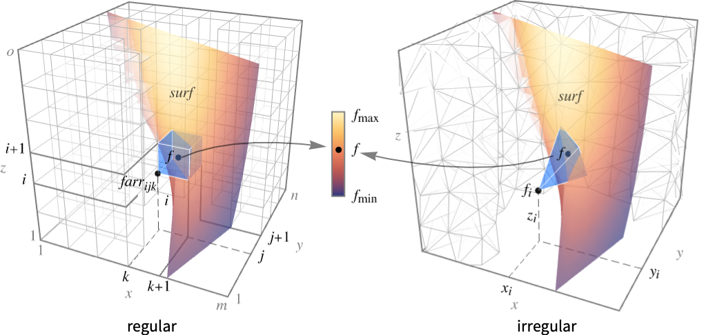
- ListSliceDensityPlot3D evaluates the interpolated function
 and maps the value to a color.
 - For regular data, the function
 has value farr[[i,j,k]] at
  .
. - For irregular data,
 has value fi at
  .
. - The plot visualizes the set
 where
where  is a color function and the region reg is the Cartesian product
  for regular data and the convex hull of {{x1,y1,z1},…,{xn,yn,zn}} for irregular data.
 - ListSliceDensityPlot3D[Tabular[…]cspec] extracts and plots values from the tabular object using the column specification cspec.
- The following forms of column specifications cspec are allowed for plotting tabular data:
-
{colx,coly,colz,colf} plot column f against columns x, y and z - The following basic slice surfaces surfi can be given:
-
Automatic automatically determine slice surfaces 
"CenterPlanes" coordinate planes through the center 
"BackPlanes" coordinate planes at the back of the plot 
"XStackedPlanes" coordinate planes stacked along  axis
axis
"YStackedPlanes" coordinate planes stacked along  axis
axis
"ZStackedPlanes" coordinate planes stacked along  axis
axis
"DiagonalStackedPlanes" planes stacked diagonally 
"CenterSphere" a sphere in the center 
"CenterCutSphere" a sphere with a cutout wedge 
"CenterCutBox" a box with a cutout octant - ListSliceDensityPlot3D[data] is equivalent to ListSliceDensityPlot3D[data,Automatic].
- The following parametrizations can be used for basic slice surfaces:
-
{"XStackedPlanes",n}, generate n equally spaced planes {"XStackedPlanes",{x1,x2,…}} generate planes for x=xi {"CenterCutSphere",ϕopen} cut angle ϕopen facing the view point {"CenterCutSphere",ϕopen,ϕcenter} cut angle ϕopen with center angle ϕcenter in  -plane
 - "YStackedPlanes", "ZStackedPlanes" follow the specifications for "XStackedPlanes", with additional features shown in the scope examples.
- The following general slice surfaces surfi can be used:
-
surfaceregion a two-dimensional region in 3D, e.g. Hyperplane volumeregion a three-dimensional region in 3D where surfi is taken as the boundary surface, e.g. Cuboid - The following wrappers can be used for slice surfaces surfi:
-
Annotation[surf,label] provide an annotation Button[surf,action] define an action to execute when the surface is clicked EventHandler[surf,…] define a general event handler for the surface Hyperlink[surf,uri] make the surface act as a hyperlink PopupWindow[surf,cont] attach a popup window to the surface StatusArea[surf,label] display in status area when the surface is moused over Tooltip[surf,label] attach an arbitrary tooltip to the surface - ListSliceDensityPlot3D has the same options as Graphics3D, with the following additions and changes: [List of all options]
-
Axes True whether to draw axes BoundaryStyle Automatic how to style surface boundaries BoxRatios {1,1,1} bounding 3D box ratios ClippingStyle None how to draw values clipped by PlotRange ColorFunction Automatic how to color the plot ColorFunctionScaling True whether to scale the arguments to ColorFunction DataRange Automatic the range of x, y, and z values to assume for data PerformanceGoal $PerformanceGoal aspects of performance to optimize PlotLegends None legends for color gradients PlotPoints Automatic approximate number of samples for the slice surfaces surfi in each direction PlotRange {Full,Full,Full,Automatic} range of f or other values to include PlotTheme $PlotTheme overall theme for the plot RegionFunction (True&) how to determine whether a point should be included ScalingFunctions None how to scale individual coordinates TargetUnits Automatic desired units to use - ColorFunction is by default supplied with the scaled value of f.
- RegionFunction is by default supplied with x, y, z, and f.
- For a farr of dimension {r,s,t}, the setting DataRangeAutomatic is equivalent to DataRange{{1,r},{1,s},{1,t}}.
- Possible settings for ScalingFunctions include:
-
sf scale the fdensity values {sx,sy,sz} scale x, y and z axes {sx,sy,sz,sf} scale x, y and z axes and fdensity values - Common built-in scaling functions s include:
-
"Log" 
log scale with automatic tick labeling "Log10" 
base-10 log scale with powers of 10 for ticks "SignedLog" 
log-like scale that includes 0 and negative numbers "Reverse" 
reverse the coordinate direction
List of all options
Examples
open all close allBasic Examples (2)
Plot the density for an array of values over a set of surfaces:
data = Table[Sqrt[x ^ 2 + y ^ 2 + z ^ 2], {z, 0, 3, 0.1}, {y, 0, 3, 0.1}, {x, 0, 3, 0.1}];ListSliceDensityPlot3D[data, "CenterPlanes"]Plot the density for an array of values on the surface ![]() :
:
data = Table[Exp[-(x ^ 2 + y ^ 2 + z ^ 2)], {z, -2, 2, .2}, {y, -2, 2, .2}, {x, -2, 2, .2}];ListSliceDensityPlot3D[data, ImplicitRegion[x ^ 3 + y ^ 2 - z ^ 2 == 0, {x, y, z}], DataRange -> {{-2, 2}, {-2, 2}, {-2, 2}}]Scope (25)
Surfaces (9)
Generate a density plot over standard slice surfaces:
data = Table[x + y + z, {z, -1, 1}, {y, -1, 1}, {x, -1, 1}];Table[ListSliceDensityPlot3D[data, sl, PlotLabel -> sl], {sl, {"CenterPlanes", "BackPlanes", "ZStackedPlanes"}}]Standard axis-aligned stacked slice surfaces:
data = Table[Sin[x] + y ^ 2 - z ^ 3, {z, -1, 1}, {y, -1, 1}, {x, -1, 1}];Table[ListSliceDensityPlot3D[data, sl, PlotLabel -> sl], {sl, {"XStackedPlanes", "YStackedPlanes", "ZStackedPlanes"}}]data = Table[Sin[x] + y ^ 2 - z ^ 3, {z, -1, 1}, {y, -1, 1}, {x, -1, 1}];Table[ListSliceDensityPlot3D[data, sl, PlotLabel -> sl], {sl, {"CenterSphere", "CenterCutSphere", "CenterCutBox"}}]Plot the densities over a half plane:
data = Table[x + y + z, {z, -1, 1}, {y, -1, 1}, {x, -1, 1}];ListSliceDensityPlot3D[data, HalfPlane[{{0, 0, 0}, {1, 0, 0}}, {0, 1, 1}]]Plotting over a volume primitive is equivalent to plotting over RegionBoundary[reg]:
data = Table[x + y + z, {z, -1, 1}, {y, -1, 1}, {x, -1, 1}];ListSliceDensityPlot3D[data, Cylinder[], DataRange -> {{-1, 1}, {-1, 1}, {-1, 1}}]Plot the densities over the surface ![]() :
:
data = Table[Sin[x y z], {z, -2, 2}, {y, -2, 2}, {x, -2, 2}];ListSliceDensityPlot3D[data, ImplicitRegion[x ^ 3 + y ^ 2 - z ^ 2 == 0, {x, y, z}], DataRange -> {{-2, 2}, {-2, 2}, {-2, 2}}]Plot the densities over multiple surfaces:
data = Table[Sin[x y z], {z, -2, 2}, {y, -2, 2}, {x, -2, 2}];ListSliceDensityPlot3D[data, {Cylinder[], "BackPlanes"}, DataRange -> {{-2, 2}, {-2, 2}, {-2, 2}}]Specify the number of stack planes:
data = Table[x + y + z, {z, -2, 2}, {y, -2, 2}, {x, -2, 2}];ListSliceDensityPlot3D[data, {"XStackedPlanes", 7}]Specify the cutting angle for a center-cut sphere slice:
data = Table[Sin[x y z], {z, -2, 2}, {y, -2, 2}, {x, -2, 2}];ListSliceDensityPlot3D[data, {"CenterCutSphere", 2Pi / 3}]Data (8)
For regular data consisting of ![]() values, the
values, the ![]() ,
, ![]() , and
, and ![]() data reflects its positions in the array:
data reflects its positions in the array:
data = Table[Sqrt[x ^ 2 + y ^ 2 + z ^ 2], {z, 0, 3, 0.1}, {y, 0, 3, 0.1}, {x, 0, 3, 0.1}];ListSliceDensityPlot3D[data, "CenterPlanes"]Provide explicit ![]() ,
, ![]() , and
, and ![]() data ranges by using DataRange:
data ranges by using DataRange:
ListSliceDensityPlot3D[data, "CenterPlanes", DataRange -> {{0, 3}, {0, 3}, {0, 3}}]Plot interpolated densities from irregular data consisting of (![]() ,
, ![]() ,
, ![]() ,
, ![]() ) tuples:
) tuples:
pts = RandomPoint[Cuboid[], 10 ^ 3];
data = Table[Append[p, p[[1]] + p[[2]] + p[[3]]], {p, pts}];ListSliceDensityPlot3D[data, "CenterPlanes"]Show the points where the data values are provided:
Show[%, Graphics3D[{AbsolutePointSize[2], Red, Point[pts]}]]Plot the density for an array of values given by SparseArray:
data = SparseArray[Table[Sqrt[x ^ 2 + y ^ 2 + z ^ 2], {z, 0, 3, 0.1}, {y, 0, 3, 0.1}, {x, 0, 3, 0.1}]]ListSliceDensityPlot3D[data]Plot the density for an array of values given by QuantityArray:
data = QuantityArray[Table[-(x ^ 2 + y ^ 2 + z ^ 2), {z, -2, 2}, {y, -2, 2}, {x, -2, 2}], "kg/m^3"];ListSliceDensityPlot3D[data, "BackPlanes", AxesLabel -> Automatic, PlotLegends -> Automatic, TargetUnits -> {"Meters", "Meters", "Meters", "g/ft^3"}]Use PlotPoints to control adaptive sampling of slice surfaces:
data = Table[Sin[π x]Sin[π y]Sin[π z], {z, -1, 1, 0.1}, {y, -1, 1, 0.1}, {x, -1, 1, 0.1}];Table[ListSliceDensityPlot3D[data, "ZStackedPlanes", PlotLabel -> pp, Axes -> False, Boxed -> False, PlotPoints -> pp], {pp, {3, 6, 9}}]Use RegionFunction to expose obscured slices:
data = Table[x ^ 2 + y ^ 2 + z ^ 2, {z, -2, 2, 0.1}, {y, -2, 2, 0.1}, {x, -2, 2, 0.1}];ListSliceDensityPlot3D[data, "ZStackedPlanes", RegionFunction -> Function[{x, y, z}, x < 0 || y > 0], DataRange -> {{-2, 2}, {-2, 2}, {-2, 2}}]ListSliceDensityPlot3D[Table[x + y + z, {z, 0, 3, 0.1}, {y, 0, 3, 0.1}, {x, 0, 3, 0.1}], "CenterPlanes", ScalingFunctions -> {"Log", None, None}]Reverse the direction of the z axis:
ListSliceDensityPlot3D[Table[x + y + z, {z, 0, 3, 0.1}, {y, 0, 3, 0.1}, {x, 0, 3, 0.1}], ImplicitRegion[x ^ 3 + y ^ 2 - z ^ 2 == 0, {x, y, z}], DataRange -> {{-2, 2}, {-2, 2}, {-2, 2}}, ScalingFunctions -> {None, None, "Reverse"}]Tabular Data (1)
tabular = Tabular[IconizedObject[«data»], {"f", "x", "y", "z"}]Plot tabular data in which each column represents data in the form {x,y,z,f}:
ListSliceDensityPlot3D[tabular -> {"x", "y", "z", "f"}]Include a legend for the plot:
ListSliceDensityPlot3D[tabular -> {"x", "y", "z", "f"}, PlotLegends -> Automatic]Presentation (7)
Use PlotTheme to immediately get overall styling:
data = Table[x ^ 2 + y ^ 2 + z ^ 2, {z, -1, 1}, {y, -1, 1}, {x, -1, 1}];Table[ListSliceDensityPlot3D[data, "CenterPlanes", PlotLabel -> t, PlotTheme -> t], {t, {"Minimal", "Scientific", "Marketing"}}]Use PlotLegends to get a color bar for the different values:
data = Table[x + y + z, {z, -1, 1}, {y, -1, 1}, {x, -1, 1}];ListSliceDensityPlot3D[data, "CenterPlanes", PlotLegends -> Automatic]Control the display of axes with Axes:
data = Table[x + y + z, {z, -1, 1}, {y, -1, 1}, {x, -1, 1}];Table[ListSliceDensityPlot3D[data, "CenterPlanes", PlotLabel -> a, Axes -> a], {a, {True, False, {True, False, True}}}]Label axes using AxesLabel and the whole plot using PlotLabel:
data = Table[x ^ 2 + y ^ 2 + z ^ 2, {z, -2, 2}, {y, -2, 2}, {x, -2, 2}];ListSliceDensityPlot3D[data, "CenterPlanes", Ticks -> None, AxesLabel -> {x, y, z}, PlotLabel -> x ^ 2 + y ^ 2 + z ^ 2]Color the plot by the function values with ColorFunction:
data = Table[x y z, {z, -1, 1}, {y, -1, 1}, {x, -1, 1}];Table[ListSliceDensityPlot3D[data, "ZStackedPlanes", PlotLabel -> c, ColorFunction -> c], {c, {Hue, "BlueGreenYellow"}}]Style the slice surface boundaries with BoundaryStyle:
data = Table[-(x ^ 2 + y ^ 2 + z ^ 2), {z, -2, 2}, {y, -2, 2}, {x, -2, 2}];ListSliceDensityPlot3D[data, "CenterPlanes", BoundaryStyle -> Gray]TargetUnits specifies which units to use in the visualization:
data = QuantityArray[Table[x ^ 2 + y ^ 2 + z ^ 2, {z, -2, 2}, {y, -2, 2}, {x, -2, 2}], "kg/m^3"];ListSliceDensityPlot3D[data, "BackPlanes", TargetUnits -> "g/ft^3", PlotLegends -> Automatic]Options (33)
BoundaryStyle (1)
BoxRatios (3)
By default, the edges of the bounding box have the same length:
data = Table[x y z, {z, -1, 2, 0.5}, {y, 0, 1, 0.5}, {x, 0, 1, 0.5}];ListSliceDensityPlot3D[data, "CenterSphere"]Use BoxRatios->Automatic to show the natural scale of the 3D coordinate values:
data = Table[x y z, {z, -1, 2, 0.5}, {y, 0, 1, 0.5}, {x, 0, 1, 0.5}];ListSliceDensityPlot3D[data, "CenterSphere", BoxRatios -> Automatic]Use custom length ratios for each side of the bounding box:
data = Table[x y z, {z, -1, 2, 0.5}, {y, 0, 1, 0.5}, {x, 0, 1, 0.5}];ListSliceDensityPlot3D[data, "CenterSphere", BoxRatios -> {1, 3, 2}]ClippingStyle (2)
data = Table[Exp[-(x ^ 2 + y ^ 2 + z ^ 2)], {z, -2, 2, 0.2}, {y, -2, 2, 0.2}, {x, -2, 2, 0.2}];ListSliceDensityPlot3D[data, "CenterPlanes", PlotRange -> {0.09, 0.72}, ClippingStyle -> {Red, Blue}]Remove clipped regions with None:
data = Table[Exp[-(x ^ 2 + y ^ 2 + z ^ 2)], {z, -2, 2, 0.2}, {y, -2, 2, 0.2}, {x, -2, 2, 0.2}];ListSliceDensityPlot3D[data, "CenterPlanes", PlotRange -> {0.09, 0.72}, ClippingStyle -> None]ColorFunction (3)
Color the slice surfaces according to the ![]() values:
values:
data = Table[x y z, {z, -1, 2, 0.5}, {y, 0, 1, 0.5}, {x, 0, 1, 0.5}];ListSliceDensityPlot3D[data, "ZStackedPlanes", ColorFunction -> Hue]Use a named color gradient available in ColorData:
data = Table[x y z, {z, -1, 2, 0.5}, {y, 0, 1, 0.5}, {x, 0, 1, 0.5}];ListSliceDensityPlot3D[data, "ZStackedPlanes", ColorFunction -> "IslandColors"]data = Table[Sin[π x], {z, -2, 2, 0.5}, {y, -2, 2, 0.5}, {x, -2, 2, 0.5}];ListSliceDensityPlot3D[data, "BackPlanes", ColorFunction -> (If[# < 0, Red, Green]&), ColorFunctionScaling -> False, DataRange -> {{-2, 2}, {-2, 2}, {-2, 2}}]ColorFunctionScaling (2)
By default, scaled values are used:
data = Table[x y z, {z, -2, 2}, {y, -2, 2}, {x, -2, 2}];ListSliceDensityPlot3D[data, "BackPlanes", ColorFunction -> Hue]Use ColorFunctionScaling->False to get access to unscaled f values:
data = Table[Sin[π x], {z, -2, 2, 0.2}, {y, -2, 2, 0.2}, {x, -2, 2, 0.2}];ListSliceDensityPlot3D[data, "BackPlanes", ColorFunction -> (If[# < 0, Red, Green]&), ColorFunctionScaling -> False, DataRange -> {{-2, 2}, {-2, 2}, {-2, 2}}]DataRange (2)
By default, the data range is taken to be the dimension of the array:
data = Table[x ^ 2 + y ^ 2 + z ^ 2, {z, -2, 2}, {y, -2, 2}, {x, -2, 2}];ListSliceDensityPlot3D[data, "YStackedPlanes"]Explicitly specify the data range:
data = Table[x ^ 2 + y ^ 2 + z ^ 2, {z, -2, 2}, {y, -2, 2}, {x, -2, 2}];ListSliceDensityPlot3D[data, "YStackedPlanes", DataRange -> {{-2, 2}, {-2, 2}, {-2, 2}}]PerformanceGoal (2)
Generate a higher-quality plot:
data = Table[x ^ 2 + y ^ 2 + z ^ 2, {z, -2, 2}, {y, -2, 2}, {x, -2, 2}];Timing[ListSliceDensityPlot3D[data, "CenterCutSphere", PerformanceGoal -> "Quality"]]Emphasize performance, possibly at the cost of quality:
data = Table[x ^ 2 + y ^ 2 + z ^ 2, {z, -2, 2}, {y, -2, 2}, {x, -2, 2}];Timing[ListSliceDensityPlot3D[data, "CenterCutSphere", PerformanceGoal -> "Speed"]]PlotLegends (3)
Show a legend for the densities:
data = Table[x ^ 2 + y ^ 2 + z ^ 2, {z, -2, 2}, {y, -2, 2}, {x, -2, 2}];ListSliceDensityPlot3D[data, "CenterPlanes", PlotLegends -> Automatic]PlotLegends automatically matches the color function:
data = Table[x ^ 2 + y ^ 2 + z ^ 2, {z, -2, 2}, {y, -2, 2}, {x, -2, 2}];ListSliceDensityPlot3D[data, "CenterPlanes", ColorFunction -> "IslandColors", PlotLegends -> Automatic]Control placement of the legend with Placed:
data = Table[Sin[x]Sin[y]Sin[z], {z, -2, 2, 0.2}, {y, -2, 2, 0.2}, {x, -2, 2, 0.2}];ListSliceDensityPlot3D[data, "BackPlanes", PlotLegends -> Placed[Automatic, Above]]PlotPoints (1)
Use PlotPoints to determine sampling of slice surfaces:
data = Table[x ^ 2 + y ^ 2 + z ^ 2, {z, -1, 1}, {y, -1, 1}, {x, -1, 1}];Table[ListSliceDensityPlot3D[data, "BackPlanes", Axes -> False, Boxed -> False, PlotPoints -> pp], {pp, {3, 5, 20}}]PlotRange (3)
Show All densities by default:
data = Table[x y z, {z, -1, 1}, {y, -1, 1}, {x, -1, 1}];ListSliceDensityPlot3D[data, "CenterSphere"]data = Table[x y z, {z, -1, 1}, {y, -1, 1}, {x, -1, 1}];ListSliceDensityPlot3D[data, "CenterSphere", PlotRange -> {All, All, {0, 2}}, BoxRatios -> Automatic, DataRange -> {{-1, 1}, {-1, 1}, {-1, 1}}]Show a select range including the ![]() values:
values:
data = Table[x y z, {z, -1, 1}, {y, -1, 1}, {x, -1, 1}];ListSliceDensityPlot3D[data, "CenterSphere", PlotRange -> {All, All, All, {0, 1}}, BoxRatios -> Automatic, DataRange -> {{-1, 1}, {-1, 1}, {-1, 1}}]PlotTheme (3)
Use a theme with detailed grid lines, ticks, and legends:
data = Table[x ^ 2 + y ^ 2 + z ^ 2, {z, -2, 2}, {y, -2, 2}, {x, -2, 2}];ListSliceDensityPlot3D[data, "CenterPlanes", PlotTheme -> "Detailed"]Override PlotTheme styles by explicitly setting options:
data = Table[x ^ 2 + y ^ 2 + z ^ 2, {z, -2, 2}, {y, -2, 2}, {x, -2, 2}];ListSliceDensityPlot3D[data, "CenterPlanes", PlotTheme -> "Detailed", FaceGrids -> None]Compare different plot themes:
data = Table[x ^ 2 + y ^ 2 + z ^ 2, {z, -2, 2}, {y, -2, 2}, {x, -2, 2}];Table[ListSliceDensityPlot3D[data, "CenterPlanes", PlotLabel -> t, PlotTheme -> t, ImageSize -> 130], {t, {"Scientific", "Monochrome", "Minimal", "Web", "Working", "Classic", "Business", "Marketing", "Detailed"}}]RegionFunction (2)
Include only the densities where ![]() or
or ![]() :
:
data = Table[x ^ 2 + y ^ 2 + z ^ 2, {z, -2, 2, 0.2}, {y, -2, 2, 0.2}, {x, -2, 2, 0.2}];ListSliceDensityPlot3D[data, "ZStackedPlanes", RegionFunction -> Function[{x, y, z}, x < 0 || y > 0], DataRange -> {{-2, 2}, {-2, 2}, {-2, 2}}]Include only the contours where ![]() :
:
data = Table[x ^ 2 + y ^ 2 + z ^ 2, {z, -2, 2}, {y, -2, 2}, {x, -2, 2}];ListSliceDensityPlot3D[data, "ZStackedPlanes", RegionFunction -> Function[{x, y, z, f}, f < 2], DataRange -> {{-2, 2}, {-2, 2}, {-2, 2}}]ScalingFunctions (5)
By default, plots have linear scales in all directions:
ListSliceDensityPlot3D[IconizedObject[«data»]]Create a plot with a log-scaled ![]() axis:
axis:
ListSliceDensityPlot3D[IconizedObject[«data»], ScalingFunctions -> {"Log", None, None}]Use ScalingFunctions to scale to reverse the coordinate direction in the ![]() direction:
direction:
ListSliceDensityPlot3D[IconizedObject[«data»], ScalingFunctions -> {None, None, "Reverse"}]Use a scale defined by a function and its inverse:
ListSliceDensityPlot3D[IconizedObject[«data»], ScalingFunctions -> {None, None, {-Log[#]&, Exp[-#]&}}]Scaling functions are applied to slices that are defined in terms of the variables:
ListSliceDensityPlot3D[IconizedObject[«data»], ImplicitRegion[x + y == 2z, {x, y, z}], ScalingFunctions -> {None, None, "Log"}]Named slice surfaces are not distorted by scaling functions:
ListSliceDensityPlot3D[IconizedObject[«data»], "CenterCutSphere", ScalingFunctions -> {None, None, "Log"}]TargetUnits (1)
Units specified by QuantityArray are converted to those specified by TargetUnits:
data = QuantityArray[Table[x ^ 2 + y ^ 2 + z ^ 2, {z, -2, 2}, {y, -2, 2}, {x, -2, 2}], "kg/m^3"];ListSliceDensityPlot3D[data, "BackPlanes", AxesLabel -> Automatic, PlotLegends -> Automatic, TargetUnits -> {"Meters", "Meters", "Meters", "g/ft^3"}]Applications (9)
Basic Data (4)
Plot density slices of data generated by ![]() :
:
data = Table[x, {z, -2, 2}, {y, -2, 2}, {x, -2, 2, 0.1}];ListSliceDensityPlot3D[data, "BackPlanes", DataRange -> {{-2, 2}, {-2, 2}, {-2, 2}}, ColorFunction -> "BrightBands"]Densities of the data generated from ![]() and
and ![]() on a sphere:
on a sphere:
{ListSliceDensityPlot3D[Table[y, {z, -2, 2}, {y, -2, 2, 0.25}, {x, -2, 2}], "BackPlanes", ColorFunction -> "BrightBands"],
ListSliceDensityPlot3D[Table[z, {z, -2, 2, 0.25}, {y, -2, 2}, {x, -2, 2}], "BackPlanes", ColorFunction -> "BrightBands"]}{ListSliceDensityPlot3D[Table[x + y, {z, -2, 2}, {y, -2, 2, 0.25}, {x, -2, 2, 0.25}], "BackPlanes", ColorFunction -> "BrightBands"],
ListSliceDensityPlot3D[Table[y + z, {z, -2, 2, 0.25}, {y, -2, 2, 0.25}, {x, -2, 2}], "BackPlanes", ColorFunction -> "BrightBands"]}{ListSliceDensityPlot3D[Table[x + y + z, {z, -2, 2, 0.25}, {y, -2, 2, 0.25}, {x, -2, 2, 0.25}], "BackPlanes", ColorFunction -> "BrightBands"],
ListSliceDensityPlot3D[Table[x - y + z, {z, -2, 2, 0.2}, {y, -2, 2, 0.2}, {x, -2, 2, 0.2}], "BackPlanes", ColorFunction -> "BrightBands"]}{ListSliceDensityPlot3D[Table[x ^ 2 + y ^ 2, {z, -2, 2}, {y, -2, 2, 0.25}, {x, -2, 2, 0.25}], "CenterPlanes"], ListSliceDensityPlot3D[Table[y ^ 2 + z ^ 2, {z, -2, 2, 0.25}, {y, -2, 2, 0.25}, {x, -2, 2}], "CenterPlanes"]}{ListSliceDensityPlot3D[Table[x ^ 2 + y ^ 2 + z ^ 2, {z, -2, 2, 0.2}, {y, -2, 2, 0.2}, {x, -2, 2, 0.2}], "CenterPlanes"], ListSliceDensityPlot3D[Table[x ^ 2 + y ^ 2 + 2z ^ 2, {z, -2, 2, 0.2}, {y, -2, 2, 0.2}, {x, -2, 2, 0.2}], "CenterPlanes"]}Data from ![]() , product of univariate functions:
, product of univariate functions:
surf = {{"XStackedPlanes", {-0.5, 0.5}}, {"ZStackedPlanes", {-0.5, 0.5}}};ListSliceDensityPlot3D[Table[Sin[π x]Sin[π y]Sin[π z], {z, -1, 1, 0.1}, {y, -1, 1, 0.1}, {x, -1, 1, 0.1}], surf, DataRange -> {{-1, 1}, {-1, 1}, {-1, 1}}]Data from ![]() and
and ![]() , univariate and bivariate functions:
, univariate and bivariate functions:
{ListSliceDensityPlot3D[Table[Sin[π x]Sin[π (y + z)], {z, -1, 1, 0.1}, {y, -1, 1, 0.1}, {x, -1, 1, 0.1}], surf, DataRange -> {{-1, 1}, {-1, 1}, {-1, 1}}], ListSliceDensityPlot3D[Table[Sin[π (x + y)]Sin[π z], {z, -1, 1, 0.1}, {y, -1, 1, 0.1}, {x, -1, 1, 0.1}], surf, DataRange -> {{-1, 1}, {-1, 1}, {-1, 1}}]}Plot density slices of the function ![]() , a trivariate function:
, a trivariate function:
ListSliceDensityPlot3D[Table[Sin[π (x + y + z)], {z, -1, 1, 0.1}, {y, -1, 1, 0.1}, {x, -1, 1, 0.1}], surf, DataRange -> {{-1, 1}, {-1, 1}, {-1, 1}}]Plot contour slices of a sum of exponentials ![]() :
:
f = Exp[-Norm[{x, y, z} - {-1, -1, -1}]^2] + Exp[-Norm[{x, y, z} - {1, 1, 1}]^2];ListSliceDensityPlot3D[Table[f, {z, -2, 2, 0.2}, {y, -2, 2, 0.2}, {x, -2, 2, 0.2}], {{"XStackedPlanes", {1, -1}}, {"ZStackedPlanes", {-1, 1}}}, DataRange -> {{-3, 3}, {-3, 3}, {-3, 3}}, BoundaryStyle -> None]Pick the points ![]() randomly in a box and plot contour slices from them:
randomly in a box and plot contour slices from them:
f = Sum[Exp[-2Norm[{x, y, z} - pi]^2], {pi, RandomPoint[Cuboid[{-1, -1, -1}, {1, 1, 1}], 10]}];data = Table[f, {z, -2, 2, 0.1}, {y, -2, 2, 0.1}, {x, -2, 2, 0.1}];p1 = ListSliceDensityPlot3D[data]Compare with other ways of visualizing:
p2 = ListDensityPlot3D[data]Show[p1, p2]Simulation Data (3)
Plot slices of a probability density function of three variables:
𝒟 = ProductDistribution[{LogNormalDistribution[0, 1], 3}];
f = PDF[𝒟, {x, y, z}]fundata = Table[f, {z, 0, 3, .1}, {y, 0, 3, .1}, {x, 0, 3, .1}];
surf = {{"XStackedPlanes", {0.1}}, {"ZStackedPlanes", {0.2}}};p1 = ListSliceDensityPlot3D[fundata, surf,
DataRange -> {{0, 3}, {0, 3}, {0, 3}}]Simulate the distribution and generate points:
pts = RandomVariate[𝒟, 10 ^ 4];Show[p1, Graphics3D[{AbsolutePointSize[2], Green, Point[pts]}]]Aggregate simulation data using histogramming:
sampdata = Last@HistogramList[RandomVariate[𝒟, 10 ^ 6], {0, 3, 0.25}];ListSliceDensityPlot3D[sampdata, surf, DataRange -> {{0, 3}, {0, 3}, {0, 3}}]Generate a Menger sponge array and plot contour slices from it:
data = Last@SubstitutionSystem[{1 -> 1 - CrossMatrix[{1, 1, 1}], 0 -> ConstantArray[0, {3, 3, 3}]}, {{{1}}}, 3];ListSliceDensityPlot3D[data, "XStackedPlanes", PlotPoints -> 50]Simulate a discrete diffusion model of a two-dimensional array of random values by averaging values of a radius-1 neighborhood in the array and plot density slices:
g[d_] := ArrayFilter[Total[#, 2] / 9&, d, 1];Time evolves along the ![]() axis, with snapshots at times 1, 3, and 7:
axis, with snapshots at times 1, 3, and 7:
simulation = NestList[g, RandomReal[1, {40, 40}], 6];ListSliceDensityPlot3D[simulation, {"ZStackedPlanes", {1, 3, 7}}, PlotLegends -> Automatic, AxesLabel -> {None, None, "time"}]Empirical Data (2)
Bin the position of atoms in a protein and plot density slices from it:
positions = ProteinData["RAB21", "AtomPositions"];{bins, data} = HistogramList[positions, 10];datarange = MinMax /@ bins;Show the concentration of atoms with the axes in picometers:
ListSliceDensityPlot3D[data, {"ZStackedPlanes", 5}, DataRange -> QuantityMagnitude[datarange], PlotRange -> {All, All, All, {10, 100}}]Visualize MRI data from a brain:
data = ExampleData[{"TestImage3D", "MRbrain"}, "GrayLevels"];ListSliceDensityPlot3D[data]Properties & Relations (5)
Use ListSliceContourPlot3D for contours on surfaces:
data = Table[x ^ 2 + y ^ 2 + z ^ 2, {z, -2, 2}, {y, -2, 2}, {x, -2, 2}];{ListSliceContourPlot3D[data, "BackPlanes"], ListSliceDensityPlot3D[data, "BackPlanes"]}Use ListDensityPlot3D for full volume visualization of the data values:
data = Table[x y z, {z, -2, 2, 0.2}, {y, -2, 2, 0.2}, {x, -2, 2, 0.2}];{ListDensityPlot3D[data], ListSliceDensityPlot3D[data, "BackPlanes"]}Use ListContourPlot3D for constant value surfaces:
data = Table[x ^ 2 + y ^ 2 + z ^ 2, {z, -2, 2}, {y, -2, 2}, {x, -2, 2}];{ListContourPlot3D[data], ListSliceDensityPlot3D[data, "CenterPlanes"]}Use SliceDensityPlot3D for functions:
data = Table[Sin[x] + y ^ 2 - z ^ 3, {z, -1, 1, 0.1}, {y, -1, 1, 0.1}, {x, -1, 1, 0.1}];{ListSliceDensityPlot3D[data, "BackPlanes"], SliceDensityPlot3D[Sin[x] + y ^ 2 - z ^ 3, "BackPlanes", {x, -1, 1}, {y, -1, 1}, {z, -1, 1}]}Use ListDensityPlot for density plots in 2D:
data = Table[x ^ 2 + y ^ 2, {z, -1, 1, 0.2}, {y, -1, 1, 0.2}, {x, -1, 1, 0.2}];{ListDensityPlot[First[data]], ListSliceDensityPlot3D[data, "BackPlanes"]}Possible Issues (1)
Slice surfaces with a constant value may appear noisy:
data = Table[x ^ 2 + y ^ 2 + z ^ 2, {z, -1, 1}, {y, -1, 1}, {x, -1, 1}];ListSliceDensityPlot3D[data, "CenterSphere"]The function ![]() is constant on the chosen slice surface:
is constant on the chosen slice surface:
ContourPlot3D[x ^ 2 + y ^ 2 + z ^ 2 == 1, {z, -1, 1}, {y, -1, 1}, {x, -1, 1}]Choosing a different slice surface gives a reasonable picture of the function:
ListSliceDensityPlot3D[data, "CenterPlanes"]Text
Wolfram Research (2015), ListSliceDensityPlot3D, Wolfram Language function, https://reference.wolfram.com/language/ref/ListSliceDensityPlot3D.html (updated 2025).
CMS
Wolfram Language. 2015. "ListSliceDensityPlot3D." Wolfram Language & System Documentation Center. Wolfram Research. Last Modified 2025. https://reference.wolfram.com/language/ref/ListSliceDensityPlot3D.html.
APA
Wolfram Language. (2015). ListSliceDensityPlot3D. Wolfram Language & System Documentation Center. Retrieved from https://reference.wolfram.com/language/ref/ListSliceDensityPlot3D.html