



SectorChart
SectorChart[{{x1,y1},{x1,y2},…}]
扇形の角度が xiと半径 yiに比例する扇形グラフを作成する.
SectorChart[{…,wi[{xi,yi},…],…,wj[{xj,yj},…],…}]
扇形の特徴が記号的ラッパー wkで定義された扇形グラフを作成する.
SectorChart[{data1,data2,…}]
複数のデータ集合 dataiから扇形グラフを作成する.
詳細とオプション
- SectorChartのデータ要素は次の形式で与えることができる.
-
{xi,yi} 純粋な扇形の角度と半径 {Quantity[xi,ux],Quantity[yi,uy]} 単位付きの扇形の角度と半径 wi[{xi,yi},…] 大きさが{xi,yi}でラッパーが wiの扇形 formi->mi メタデータ miを持った扇形の形式 - これらの形式で与えられないデータは扇形グラフの作成時に無視される.
- SectorChartのためのデータ集合は次の形式で与えることができる.
-
{e1,e2,…} ラッパーがある/ない要素のリスト <k1e1,k2e2,…> キーと長さの連想 TimeSeries[…],EventSeries[…],TemporalData[…] 時系列,事象系列,一時データ WeightedData[…] 重みの付いたデータ集合 w[{e1,e2,…},…] データ集合全体に適用されたラッパー w[{data1,data1,…},…] すべてのデータ集合に適用されたラッパー - SectorChart[objcspec]は,列指定 cspec を用いて,Tabularオブジェクト,TimeSeriesオブジェクト,またはEventSeriesオブジェクト obj から値を抽出してプロットする.
- 次は,表データのプロットに使用可能な列指定 cspec の形式である.
-
{colx,coly} 列 y と列 x をプロットする {{colx1,coly1},{colx2,coly2},…} 列 y1,列x1, y2,x2, …をプロットする - グラフの要素に次のラッパーを使用することができる.
-
Annotation[e,label] 注釈を与える Button[e,action] 要素がクリックされたときに実行するアクションを定義する Callout[e,label] コールアウトを付けて要素を表示する EventHandler[e,…] 要素の一般的なイベントハンドラを定義する Hyperlink[e,uri] 要素がハイパーリンクとして機能するようにする Labeled[e,…] 要素にラベルを付けて表示する Legended[e,…] グラフの説明文に要素の特徴を含む Mouseover[e,over] 要素がマウスオーバーの形式を示すようにする PopupWindow[e,cont] 要素にポップアップウィンドウを加える StatusArea[e,label] 要素の上にマウスが来たときにステータスエリアに表示する Style[e,opts] 要素を指定したスタイルで示す Tooltip[e,label] 要素に任意のツールチップを加える - SectorChartでは,Labeled,Callout,Placedで次の位置が取れる.
-
"RadialOuter","RadialCenter","RadialInner" 扇形内の位置 "RadialOutside","RadialInside","RadialEdge" 扇形外の位置 "RadialCallout" 対象物を線で示した位置 {{sθ,sr},{lx,ly}} 扇形内のスケールされた位置{sθ,sr}におけるラベル内のスケールされた位置{lx,ly} - SectorChartのCalloutには次の位置 pos を使うことができる.
-
Automatic 自動的に置く {x,y} グラフィックス内の位置 Scaled[{sθ,sr}] 扇形内のスケールされた極位置{sθ,sr} {pos,{lx,ly}} 位置 pos のラベル内のスケールされた位置{lx,ly} - SectorChartにはGraphicsと同じオプションに次の追加・変更を加えたものが使える. [全オプションのリスト]
-
ChartElementFunction Automatic 扇形の生のグラフィックスをどのように生成するか ColorFunction Automatic 扇形の彩色方法 ColorFunctionScaling True ColorFunctionの引数を正規化するかどうか LabelingFunction Automatic 扇形にどのようにラベルを付けるか LabelingSize Automatic コールアウトとラベルの最大サイズ LegendAppearance Automatic 凡例の全体的な外観 PerformanceGoal $PerformanceGoal パフォーマンスのどの面について最適化するか PlotInteractivity $PlotInteractivity インタラクティブ要素を許可するかどうか PlotLabels None 扇形のカテゴリラベル PlotLayout Automatic 使用する全体的なレイアウト PlotLegends None データ要素とデータ集合の凡例 PlotRange Automatic 含める値の範囲 PlotStyle Automatic 扇形のスタイル PlotTheme $PlotTheme グラフの全体的なテーマ PolarAxes False 極座標軸をどのように描くか PolarAxesOrigin Automatic 極座標軸をどこに描くか PolarGridLines None 描くべき極格子 PolarTicks Automatic 極座標軸の目盛 SectorOrigin Automatic 扇形の初期角度と半径 SectorSpacing Automatic 扇形の間隔 TargetUnits Automatic グラフ内に表示する単位 - PlotLayoutの次の設定を使って複数のデータ集合を単一のパネルに表示できる.
-

"Grouped" 各データ集合のデータを分離する 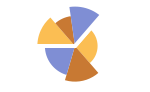
"Stacked" 各データ集合のデータを積み重ねる - 次は,個々のデータ集合を異なるパネルに表示する際のPlotLayoutの可能な設定である.
-
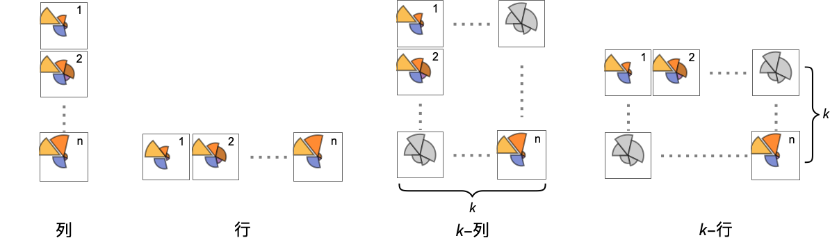
"Column" 異なる扇形のグループをパネルの列に使う "Row" 異なる扇形のグループをパネルの行に使う {"Column",k},{"Row",k} k 列(または行)を使う {"Column",UpTo[k]},{"Row",UpTo[k]} 最高で k 列(または行)を使う - PlotLegendsに対する典型的な設定には,次のものが含まれる.
-
None 凡例なし Automatic 凡例を自動的に決定する {lbl1,lbl2,…} lbl1,lbl2,…を凡例ラベルとして用いる Placed[lspec,…] 凡例の配置を指定する - PlotStylesty は,各曲線に使用するスタイルを指定する.取り得る設定には,次のものが含まれる.
-
{sty1,sty2,…} データに対するスタイルの列 <"key"val,…> データの異なるレベルに対するスタイル要素 - 使用可能なキーは次の通りである.
-
"Base" すべての棒に対する全体的なスタイル "Elements" 各グループ内の要素 yiに対するスタイルのリスト "Groups" 値 dataiの各グループに対するスタイルのリスト - ColorData["DefaultChartColors"]は,PlotStyleによって使用されるデフォルトの色の並びを与える.
- ChartElementFunctionに渡される引数は,ネストしたデータ集合リストにおける各レベルからの扇形の範囲{{θmin,θmax},{rmin,rmax}},値{xi,yi},メタデータ{m1,m2,…}である.
- ChartElementFunctionの組込み設定のリストはChartElementData["SectorChart"]で得られる.
- ColorFunctionに渡される引数は θ と r である.ただし,θ は扇形の角度,r は半径である.
- SectorChartのオプションおよびその他の構造からのスタイルその他の指定は事実上ChartStyle,ColorFunction,Styleその他のラッパー,ChartElementFunctionの順に適用される.後ろの指定が前の指定を無効にする.
全オプションのリスト
例題
すべて開く すべて閉じる例 (4)
SectorChart[{{1, 1}, {1, 2}, {1, 3}}]SectorChart[{{1, 1}, {1, 2}, {1, 3}}, SectorOrigin -> {Automatic, 1}]SectorChart[{{{1, 1}, {1, 2}, {1, 3}}, {{7, 3}, {5, 2}, {1, 1}}}]SectorChart[{{{1, 1}, {1, 2}, {1, 3}}, {{7, 3}, {5, 2}, {1, 1}}}, ChartLayout -> "Row"]SectorChart[{{1, 1}, {1, 2}, {1, 3}}, PlotLabels -> {"a", "b", "c"}]SectorChart[{{1, 1}, {1, 2}, {1, 3}}, PlotLegends -> {"a", "b", "c"}]スコープ (32)
データとレイアウト (13)
SectorChart[{{{1, 1}, {1, 2}, {1, 3}}, {{2, 1}, {2, 2}, {2, 3}}, {{3, 1}, {3, 2}, {3, 3}}}]SectorChart[{{{1, 2}, {2, 3}}, {{1, 1}, {2, 2}, {3, 3}}, {{1, 1}, {2, 2}, {3, 3}, {4, 4}}}]実数ではないデータは欠測値とみなされ,一般にグラフからは除かれる:
SectorChart[{{{1, 2}, {2, 3}}, {{1, 1}, {2, Missing[]}, {3, 3}}, {{1, 1}, {2, 2}, {foo, 3}, {4, 4}}}]SectorChart[{{Quantity[1, "Seconds"], Quantity[2, "Meters"]}, {Quantity[1, "Seconds"], Quantity[3, "Meters"]}, {Quantity[2, "Seconds"], Quantity[5, "Meters"]}, {Quantity[3, "Seconds"], Quantity[7, "Meters"]}, {Quantity[5, "Seconds"], Quantity[11, "Meters"]}}]TimeSeries,EventSeries,TemporalDataにおけるタイムスタンプは無視される:
SectorChart[TimeSeries[{{19, 16}, {9, 3}, {7, 2}, {17, 5}}, {"May 24, 1982"}]]SectorChart[<|"a" -> {2, 3}, "b" -> {4, 6}, "c" -> {5, 8}, "d" -> {3, 7}|>]SectorChart[<|"a" -> {2, 3}, "b" -> {4, 6}, "c" -> {5, 8}, "d" -> {3, 7}|>, PlotLabels -> Placed[Automatic, "RadialCallout"]]SectorChart[<|"a" -> {2, 3}, "b" -> {4, 6}, "c" -> {5, 8}, "d" -> {3, 7}|>, PlotLabels -> Callout[Automatic]]SectorChart[<|"a" -> {2, 3}, "b" -> {4, 6}, "c" -> {5, 8}, "d" -> {3, 7}|>, PlotStyle -> {Hue[0.61, 0.7, 1], Hue[0.17, 0.4, 0.65], Hue[0.64, 0.5, 0.75], Hue[0.45, 0.4, 0.7]}, PlotLegends -> Automatic]SectorChart[<|"group a" -> <|"a" -> {1, 1}, "b" -> {2, 3}, "c" -> {5, 8}, "d" -> {3, 7}|>, "group b" -> <|"a" -> {1, 1}, "b" -> {3, 2}, "c" -> {5, 3}, "d" -> {7, 2}|>|>, PlotLegends -> Automatic]WeightedData中の重みは無視される:
SectorChart[WeightedData[{{1, 2}, {3, 4}, {5, 6}}, {0.5, 0.2, 0.1}]]Table[SectorChart[RandomInteger[{1, 4}, {2, 10, 2}], ChartLayout -> l], {l, {"Grouped", "Stacked"}}]SectorChart[{IconizedObject[«data #1»], IconizedObject[«data #2»], IconizedObject[«data #3»]}, ImageSize -> Medium, ChartLayout -> "Row"]SectorChart[{IconizedObject[«data #1»], IconizedObject[«data #2»], IconizedObject[«data #3»]}, ImageSize -> Medium, ChartLayout -> "Column"]SectorChart[{IconizedObject[«data #1»], IconizedObject[«data #2»], IconizedObject[«data #3»], IconizedObject[«data #4»]}, ImageSize -> Medium, ChartLayout -> {"Row", 2}]Table[SectorChart[{{1, 1}, {1, 2}, {2, 3}, {3, 2}}, SectorOrigin -> o, PlotLabel -> o], {o, {{Pi / 6, "Clockwise"}, {Pi / 6, "Counterclockwise"}}}]Table[SectorChart[{{1, 1}, {1, 2}, {2, 3}, {3, 2}}, SectorOrigin -> o, PlotLabel -> o], {o, {0, Pi / 2}}]Table[SectorChart[{{1, 1}, {1, 2}, {2, 3}, {3, 2}}, SectorOrigin -> o, PlotLabel -> o], {o, {{{0, "Clockwise"}, 0}, {{0, "Clockwise"}, 1}}}]Table[SectorChart[{{{2, 1}, {3, 4}, {4, 2}, {3, 4}}, {{2, 2}, {2, 3}, {3, 2}, {4, 3}}}, SectorSpacing -> s, PlotLabel -> s], {s, {Automatic, {0, 1}, {0.1, 1}}}]表形式データ (3)
tabdata = AggregateRows[Tabular[ResourceData["Sample Data: 1993 US Cars"]], {"AvgPrice" -> (Mean[#AvgPrice]&), "TotalCars" -> (Length[#AvgPrice]&), "AvgWeight" -> (Mean[#Weight]&), "AvgFuelTankCap" -> (Mean[#FuelTankCapacity]&)}, {"Type"}]SectorChart[tabdata -> {"TotalCars", "AvgPrice"}, PlotLabels -> Normal[tabdata[All, "Type"]]]TimeSeriesまたはEventSeriesのすべての成分の値をプロットする:
SectorChart[TimeSeries[TimeEventSeries`TimestampData[Association["UniformlySpacedQ" -> True, "Count" -> 5,
   "Endpoints" -> TabularColumn[Association[
      "Data" -> {2, {{NumericArray[{20563, -2147483648}, "Integer32"], {},
          DataStructure["BitVec ... {{TabularColumn[Association["Data" -> {{1, 3, 5, 7, 8}, {}, None},
           "ElementType" -> "Integer64"]], TabularColumn[Association[
           "Data" -> {{13, 17, 18, 19, 19}, {}, None}, "ElementType" -> "Integer64"]]}}]]]],
Association[]]]TimeSeriesまたはEventSeriesの成分ペアの値をプロットする:
ts = TimeSeries[TimeEventSeries`TimestampData[Association["UniformlySpacedQ" -> True, "Count" -> 5,
   "Endpoints" -> TabularColumn[Association[
      "Data" -> {2, {{NumericArray[{20563, -2147483648}, "Integer32"], {},
          DataStructure["BitVec ... olumn[Association[
           "Data" -> {{10, 10, 14, 16, 18}, {}, None}, "ElementType" -> "Integer64"]],
         TabularColumn[Association["Data" -> {{13, 10, 6, 6, 6}, {}, None},
"ElementType" -> "Integer64"]]}}]]]], Association[]];SectorChart[ts -> {"a", "b"}]SectorChart[ts -> {{"a", "b"}, {"a", "c"}}]ラッパー (4)
個々のデータ,データ集合,あるいはデータ集合の集合にラッパーを使う:
{{d1, d2, d3, d4}, {w1, w2, w3, w4}} = {{{2, 1}, {3, 4}, {4, 2}, {3, 4}}, {{2, 2}, {2, 3}, {3, 2}, {4, 3}}};{SectorChart[{{d1, Style[d2, RGBColor[0.93, 0.27, 0.27]], d3, d4}, {w1, w2, w3, w4}}], SectorChart[{Style[{d1, d2, d3, d4}, RGBColor[0.14, 0.8, 0.14]], {w1, w2, w3, w4}}], SectorChart[Style[{{d1, d2, d3, d4}, {w1, w2, w3, w4}}, RGBColor[0.4, 0.6, 1]]]}{SectorChart[{{d1, Style[d2, RGBColor[0.93, 0.27, 0.27]], d3, d4}, {w1, w2, w3, w4}}], SectorChart[{Style[{d1, Style[d2, RGBColor[0.93, 0.27, 0.27]], d3, d4}, RGBColor[0.14, 0.8, 0.14]], {w1, w2, w3, w4}}], SectorChart[Style[{Style[{d1, Style[d2, RGBColor[0.93, 0.27, 0.27]], d3, d4}, RGBColor[0.14, 0.8, 0.14]], {w1, w2, w3, w4}}, RGBColor[0.4, 0.6, 1]]]}SectorChart[{{1, 3}, {2, 1}, Tooltip[{3, 3}, "median"], {4, 2}}]SectorChart[Table[Tooltip[{QuantityMagnitude@CountryData[c, "Population"], QuantityMagnitude@CountryData[c, "LifeExpectancy"]}, CountryData[c, "Flag"]], {c, CountryData["G8"]}]]PopupWindowを使って追加的なドロップダウン情報を与える:
SectorChart[{{1, 3}, {2, 1}, PopupWindow[{3, 3}, DateListPlot[FinancialData["IBM", "Jan. 1, 2004"]]], {4, 2}}]Buttonを使って任意のアクションを開始することができる:
SectorChart[{{1, 3}, {2, 1}, Button[{3, 3}, Speak[3]], {4, 2}}]スタイルと外観 (5)
SectorChart[{{1, 3}, {2, 1}, {3, 3}, {4, 2}}, PlotStyle -> {RGBColor[0.93, 0.27, 0.27], RGBColor[0.14, 0.8, 0.14], RGBColor[0.4, 0.6, 1], RGBColor[1, 0.75, 0]}]{SectorChart[{{1, 3}, {2, 1}, {3, 3}, {4, 2}}, PlotTheme -> "Web"], SectorChart[{{1, 3}, {2, 1}, {3, 3}, {4, 2}}, PlotTheme -> "Marketing"], SectorChart[{{1, 3}, {2, 1}, {3, 3}, {4, 2}}, PlotTheme -> "Monochrome"]}ChartElementData["SectorChart"]Table[SectorChart[{{1, 3}, {2, 1}, {3, 3}, {4, 2}}, ChartElementFunction -> f, PlotStyle -> {RGBColor[0.761959, 0.470832, 0.940597], RGBColor[0.927848, 0.742785, 0.6151383333333333], RGBColor[0.929162, 0.95034, 0.6648153333333333], RGBColor[0.431296, 0.709773, 0.927077]}], {f, {"NoiseSector", "PlateauSector"}}]詳細設定には「パレット」▶「チャートエレメントスキーム」を使う:
SectorChart[{{1, 3}, {2, 1}, {3, 3}, {4, 2}}, ChartElementFunction -> ChartElementDataFunction["GlassSector", "GradientDirection" -> "Angular"], PlotStyle -> {RGBColor[0.468742, 0., 0.0158236], RGBColor[0.871407, 0.20684366666666665, 0.013399966666666667], RGBColor[0.9899876666666667, 0.5566463333333334, 0.06420996666666667], RGBColor[1., 0.820127, 0.126955]}]SectorChart[{{1, 3}, {2, 2}, {3, 3}, {4, 2}}, PlotTheme -> "Marketing"]SectorChart[{{{4, 9}, {7, 4}, {4, 10}, {7, 4}, {4, 9}}, {{7, 4}, {5, 7}, {9, 8}, {8, 4}, {9, 4}}}, PlotTheme -> "Monochrome"]ラベルと凡例 (7)
Labeledを使って扇形にラベルを付ける:
SectorChart[{{1, 3}, {2, 1}, Labeled[{3, 3}, "label"], {4, 2}}]Table[SectorChart[{{1, 3}, {2, 1}, Labeled[{3, 3}, "label", p], {4, 2}}, PlotLabel -> p, SectorOrigin -> {Automatic, 1}], {p, {"RadialInner", "RadialCenter", "RadialOuter"}}]Table[SectorChart[{{1, 3}, {2, 1}, Labeled[{3, 3}, "label", p], {4, 2}}, PlotLabel -> p, SectorOrigin -> {Automatic, 1}], {p, {"RadialInside", "RadialOutside"}}]Table[SectorChart[{Labeled[{1, 3}, "L1", p], Labeled[{2, 1}, "L2", p], Labeled[{3, 3}, "L3", p], Labeled[{4, 2}, "L4", p]}, PlotLabel -> p], {p, {"RadialCallout", "VerticalCallout"}}]Calloutを使って扇形にラベルを加える:
SectorChart[{{2, 1}, Callout[{2, 3}, "label"], {3, 4}}]SectorChart[{{2, 1}, Callout[{2, 3}, "label", Appearance -> "Balloon"], {3, 4}}]SectorChart[Callout[#, Unique["text"]]& /@ RandomReal[{0.3, 1}, {6, 2}]]LabelingFunctionを使って扇形の値のラベルを与える:
SectorChart[{{2, 1}, {2, 3}, {3, 4}, {4, 2}}, LabelingFunction -> "RadialOutside"]SectorChart[RandomInteger[{3, 10}, {6, 2}], LabelingFunction -> (Callout[Style[Total@#, 10 + #[[2]]], Automatic]&)]オプション (82)
AspectRatio (4)
SectorChart[{{1, 3}, {2, 1}, {3, 3}, {4, 2}}]AspectRatio1として高さと幅を等しくする:
SectorChart[{{1, 3}, {2, 1}, {3, 3}, {4, 2}}, AspectRatio -> 1]SectorChart[{{1, 3}, {2, 1}, {3, 3}, {4, 2}}, AspectRatio -> 1 / 2]AspectRatioFullとすると,他の構造物内にぴったり納まるように高さと幅が調整される:
plot = SectorChart[{{1, 3}, {2, 1}, {3, 3}, {4, 2}}, AspectRatio -> Full];{Framed[Pane[plot, {50, 100}]], Framed[Pane[plot, {100, 100}]], Framed[Pane[plot, {100, 50}]]}Axes (3)
デフォルトで,Axesは描かれない:
SectorChart[{{1, 3}, {2, 1}, {3, 3}, {4, 2}}]SectorChart[{{1, 3}, {2, 1}, {3, 3}, {4, 2}}, Axes -> True]{SectorChart[{{1, 3}, {2, 1}, {3, 3}, {4, 2}}, Axes -> {True, False}], SectorChart[{{1, 3}, {2, 1}, {3, 3}, {4, 2}}, Axes -> {False, True}]}AxesLabel (3)
SectorChart[{{1, 3}, {2, 1}, {3, 3}, {4, 2}}, Axes -> True]

SectorChart[{{1, 3}, {2, 1}, {3, 3}, {4, 2}}, Axes -> True, AxesLabel -> label]SectorChart[{{1, 3}, {2, 1}, {3, 3}, {4, 2}}, Axes -> True, AxesLabel -> {x, y}]AxesOrigin (2)
AxesStyle (3)
SectorChart[{{1, 3}, {2, 1}, {3, 3}, {4, 2}}, Axes -> True, AxesStyle -> RGBColor[0.93, 0.27, 0.27]]SectorChart[{{1, 3}, {2, 1}, {3, 3}, {4, 2}}, Axes -> True, AxesStyle -> {{Thick, RGBColor[0.93, 0.27, 0.27]}, {Thick, RGBColor[0.4, 0.6, 1]}}]SectorChart[{{1, 3}, {2, 1}, {3, 3}, {4, 2}}, Axes -> True, AxesStyle -> RGBColor[0.14, 0.8, 0.14], TicksStyle -> RGBColor[0.93, 0.27, 0.27]]ChartElementFunction (5)
ChartElementFunctionの組込み設定のリストを得る:
ChartElementData["SectorChart"]詳細設定には「パレット」▶「チャートエレメントスキーム」を使う:
Table[SectorChart[Tuples[{1, 2}, 2], ChartElementFunction -> f, PlotStyle -> {RGBColor[0.761959, 0.470832, 0.940597], RGBColor[0.927848, 0.742785, 0.6151383333333333], RGBColor[0.929162, 0.95034, 0.6648153333333333], RGBColor[0.431296, 0.709773, 0.927077]}, PlotLabel -> f], {f, {"Sector", "PlateauSector"}}]Table[SectorChart[Tuples[{1, 2}, 2], ChartElementFunction -> f, PlotStyle -> {RGBColor[0.761959, 0.470832, 0.940597], RGBColor[0.927848, 0.742785, 0.6151383333333333], RGBColor[0.929162, 0.95034, 0.6648153333333333], RGBColor[0.431296, 0.709773, 0.927077]}, PlotLabel -> f], {f, {"NoiseSector", "OscillatingSector"}}]Table[SectorChart[Tuples[{1, 2}, 2], ChartElementFunction -> f, PlotStyle -> {RGBColor[0.761959, 0.470832, 0.940597], RGBColor[0.927848, 0.742785, 0.6151383333333333], RGBColor[0.929162, 0.95034, 0.6648153333333333], RGBColor[0.431296, 0.709773, 0.927077]}, PlotLabel -> f], {f, {"SquareWaveSector", "TriangleWaveSector"}}]Table[SectorChart[Tuples[{1, 2}, 2], ChartElementFunction -> f, PlotStyle -> {RGBColor[0.761959, 0.470832, 0.940597], RGBColor[0.927848, 0.742785, 0.6151383333333333], RGBColor[0.929162, 0.95034, 0.6648153333333333], RGBColor[0.431296, 0.709773, 0.927077]}, PlotLabel -> f], {f, {"GlassSector", "GradientSector"}}]ChartElementDataを使って上記と同じグラフ要素描画関数を指定する:
SectorChart[Tuples[{1, 2}, 2], ChartElementFunction -> Function[{angleRadiusMinMax, yr, meta}, ChartElementData["TriangleWaveSector"][angleRadiusMinMax, yr, meta]]]カスタマイズされたChartElementFunctionを書く:
f[{{t0_, t1_}, {r0_, r1_}}, ___] := Disk[{0, 0}, r1, {t0, t1}]SectorChart[Tuples[{1, 2}, 2], ChartElementFunction -> f]入力から渡されたメタデータ,この場合はデータのグラフ化を使う:
DataDrilldownSector[{{t0_, t1_}, {r0_, r1_}}, y_, {data_List}] :=
PopupWindow[ChartElementData["NoiseSector"][{{t0, t1}, {r0, r1}}, y], BarChart[data]]DataDrilldownSector[{{t0_, t1_}, {r0_, r1_}}, y_, _] :=
ChartElementData["Sector"][{{t0, t1}, {r0, r1}}, y]SectorChart[{{1, 1} -> Range[5], {1, 2}, {2, 1} -> RandomReal[1, 10], {2, 2}}, ChartElementFunction -> DataDrilldownSector]ColorFunction (4)
SectorChart[Table[{Exp[-t ^ 2], Exp[-t ^ 2]}, {t, -2, 2, 0.25}], ColorFunction -> Function[{angle, radius}, ColorData["Rainbow"][angle]]]ColorFunctionScaling->Falseを使ってスケールされていない角の値を得る:
SectorChart[Tuples[{1, 2}, 2], ColorFunction -> (Switch[{#1, #2}, {1, 1}, RGBColor[1, 0.75, 0], {1, 2}, RGBColor[0.98, 0.56, 0.17], {2, 1}, RGBColor[0.93, 0.27, 0.27], _, RGBColor[0.4, 0.6, 1]]&), ColorFunctionScaling -> False]SectorChart[{{1, 1}, {1, 2}, {2, 1}, {2, 2}}, ColorFunction -> Function[{angle, radius}, ColorData["Rainbow"][angle radius / 4]], ColorFunctionScaling -> False]ColorFunctionはPlotStyleのスタイルを無効にする:
SectorChart[Tuples[{1, 2, 3}, 2], PlotStyle -> {RGBColor[0.93, 0.27, 0.27], RGBColor[0.14, 0.8, 0.14], RGBColor[0.67, 0.54, 0.42]}, ColorFunction -> "Pastel"]ColorFunctionを使って異なるスタイル効果を組み合せる:
SectorChart[Table[{Exp[-t ^ 2], Exp[-t ^ 2]}, {t, -2, 2, 0.25}], ColorFunction -> Function[{angle, radius}, Opacity[radius]], PlotStyle -> RGBColor[0.8, 0.3, 0.8]]ColorFunctionScaling (2)
ColorFunctionScaling->Falseを使ってスケールされていない高さの値を得る:
SectorChart[Tuples[{1, 2}, 2], ColorFunction -> (Switch[{#1, #2}, {1, 1}, RGBColor[1, 0.75, 0], {1, 2}, RGBColor[0.98, 0.56, 0.17], {2, 1}, RGBColor[0.93, 0.27, 0.27], _, RGBColor[0.4, 0.6, 1]]&), ColorFunctionScaling -> False]SectorChart[{{1, 1}, {1, 2}, {2, 1}, {2, 2}}, ColorFunction -> Function[{angle, radius}, ColorData["Rainbow"][angle radius / 4]], ColorFunctionScaling -> False]Frame (4)
SectorChartは,デフォルトで,枠を使わない:
SectorChart[{{1, 3}, {2, 1}, {3, 3}, {4, 2}}]SectorChart[{{1, 3}, {2, 1}, {3, 3}, {4, 2}}, Frame -> True]SectorChart[{{1, 3}, {2, 1}, {3, 3}, {4, 2}}, Frame -> {{True, True}, {False, False}}]SectorChart[{{1, 3}, {2, 1}, {3, 3}, {4, 2}}, Frame -> {{True, False}, {True, False}}]FrameLabel (4)
SectorChart[{{1, 3}, {2, 1}, {3, 3}, {4, 2}}, Frame -> True, FrameLabel -> {"label"}]SectorChart[{{1, 3}, {2, 1}, {3, 3}, {4, 2}}, Frame -> True, FrameLabel -> {"bottom", "left"}]SectorChart[{{1, 3}, {2, 1}, {3, 3}, {4, 2}}, Frame -> True, FrameLabel -> {{"left", "right"}, {"bottom", "top"}}]SectorChart[{{1, 3}, {2, 1}, {3, 3}, {4, 2}}, Frame -> True, FrameLabel -> {{"left", "right"}, {"bottom", "top"}}, LabelStyle -> Directive[Bold, RGBColor[0.67, 0.54, 0.42]]]FrameStyle (2)
SectorChart[{{1, 3}, {2, 1}, {3, 3}, {4, 2}}, Frame -> True, FrameStyle -> Directive[RGBColor[0.67, 0.54, 0.42], Thick]]SectorChart[{{1, 3}, {2, 1}, {3, 3}, {4, 2}}, Frame -> True, FrameStyle -> {{Directive[RGBColor[0.14, 0.8, 0.14], Thick], RGBColor[0.93, 0.27, 0.27]}, {Directive[GrayLevel[0.62], Thick], RGBColor[0.4, 0.6, 1]}}]ImageSize (7)
Tiny,Small,Medium,Largeのような名前付きのサイズを使う:
{SectorChart[{{1, 1}, {1, 2}, {1, 3}}, ImageSize -> Tiny], SectorChart[{{1, 1}, {1, 2}, {1, 3}}, ImageSize -> Small]}SectorChart[{{1, 1}, {1, 2}, {1, 3}}, ImageSize -> 150]SectorChart[{{1, 1}, {1, 2}, {1, 3}}, ImageSize -> {Automatic, 150}]SectorChart[{{1, 1}, {1, 2}, {1, 3}}, ImageSize -> UpTo[200]]SectorChart[{{1, 1}, {1, 2}, {1, 3}}, ImageSize -> {200, 250}, Background -> LightBlue]SectorChart[{{1, 1}, {1, 2}, {1, 3}}, ImageSize -> {UpTo[250], UpTo[200]}]ImageSizeFullを使ってオブジェクト内の使用可能な空間を埋める:
chart = SectorChart[{{1, 1}, {1, 2}, {1, 3}}, ImageSize -> Full];{Framed[Pane[chart, {100, 100}]], Framed[Pane[chart, {200, 200}]]}Framed[Pane[SectorChart[{{1, 1}, {1, 2}, {1, 3}}, ImageSize -> {Scaled[0.5], Scaled[0.5]}, Background -> LightBlue], {200, 100}]]LabelingFunction (8)
TooltipとStatusAreaからの値で自動的なラベル付けを使う:
SectorChart[{{1, 1}, {1, 2}, {2, 3}, {3, 2}}, LabelingFunction -> Automatic]SectorChart[{{1, 1}, {1, 2}, {2, 3}, {3, 2}}, LabelingFunction -> None]Placedを使ってラベルの置き方を制御する:
Table[SectorChart[{{1, 1}, {1, 2}, {2, 3}, {3, 2}}, LabelingFunction -> (Placed[#, p]&), PlotLabel -> p, Ticks -> None], {p, {"RadialInner", "RadialCenter", "RadialOuter"}}]Table[SectorChart[{{1, 1}, {1, 2}, {2, 3}, {3, 2}}, SectorOrigin -> {Automatic, 4}, LabelingFunction -> (Placed[#, p]&), PlotLabel -> p], {p, {"RadialInside", "RadialOutside", "RadialEdge"}}]Table[SectorChart[{{1, 1}, {1, 2}, {2, 3}, {3, 2}}, LabelingFunction -> (Placed[#, p]&), PlotLabel -> p], {p, {"RadialCallout", "VerticalCallout"}}]Table[SectorChart[{{1, 1}, {1, 2}, {2, 3}, {3, 2}}, LabelingFunction -> (Placed[#, p]&), PlotLabel -> p, SectorOrigin -> {Automatic, 2}], {p, {{0.1, 0.1}, {1 / 2, 1 / 2}, {1, 1}}}]Calloutを使って自動的にラベルを置く:
SectorChart[{{1, 1}, {1, 2}, {2, 3}, {3, 2}}, LabelingFunction -> (Callout[Row[{"$", NumberForm[#[[2]], {2, 2}]}], Automatic]&)]SectorChart[{{1, 1}, {1, 2}, {2, 3}, {3, 2}}, LabelingFunction -> (Placed[Row[{"$", #[[1]]}, " "], "RadialOutside"]&)]data = {{{1, 1}, {1, 2}, {2, 3}, {3, 2}}, {{1, 1}, {2, 2}, {2, 3}}};SectorChart[data, PlotLabels -> {{"r1", "r2"}, {"c1", "c2", "c3"}}, LabelingFunction -> (Placed[Row[{#3[[1, 1]], #3[[2, 1]], #1}, ","], Tooltip]&)]LabelingSize (3)
SectorChart[{{1, 1}, {1, 2}, {2, 3}, {3, 2}}, PlotLabels -> {"healthfulness", "obstreperous", "spectrogram", "vestige"}]SectorChart[{{1, 1}, {1, 2}, {2, 3}, {3, 2}}, PlotLabels -> {[image], [image], [image], [image], [image], [image], [image]}]SectorChart[{{1, 1}, {1, 2}, {2, 3}, {3, 2}}, PlotLabels -> {"healthfulness", "obstreperous", "spectrogram", "vestige"}, LabelingSize -> 50]PlotInteractivity (4)
扇形の数がそれほど多くないグラフには,ツールチップとマウスオーバー効果が自動的に付けられる:
SectorChart[{{1, 1}, {2, 1}, {2, 2}}]SectorChart[{{1, 1}, {2, 1}, {2, 2}}, PlotInteractivity -> False]入力の一部として与えられたインタラクティブ要素を無効にする:
SectorChart[{{1, 1}, {2, 1}, Tooltip[{2, 2}, "Hello"]}, PlotInteractivity -> False]与えたインタラクティブ要素は有効にして,自動のものは無効にする:
SectorChart[{{1, 1}, {2, 1}, Tooltip[{2, 2}, "Hello"]}, PlotInteractivity -> <|"User" -> True, "System" -> False|>]PlotLabels (8)
SectorChart[{{1, 1}, {1, 2}, {2, 3}, {3, 2}}, PlotLabels -> {"a", "b", "c", "d"}]SectorChart[{{{1, 2}, {1, 3}, {1, 2}}, {{2, 2}, {1, 1}, {3, 2}}}, PlotLabels -> {"a", "b"}]データ内のLabeledラッパーは,追加のラベルを配置する:
SectorChart[{{1, 1}, Labeled[{1, 2}, "label", "RadialOutside"], {2, 3}, {3, 2}}, PlotLabels -> {"a", "b", "c", "d"}]Placedを用いてラベルの配置を制御する:
Table[SectorChart[{{1, 1}, {1, 2}, {2, 3}, {3, 2}}, PlotLabels -> Placed[{"a", "b", "c", "d"}, p], PlotLabel -> p], {p, {"RadialInner", "RadialCenter", "RadialOuter"}}]Table[SectorChart[{{1, 1}, {1, 2}, {2, 3}, {3, 2}}, SectorOrigin -> {Automatic, 1}, PlotLabels -> Placed[{"a", "b", "c", "d"}, p], PlotLabel -> p, Ticks -> None], {p, {"RadialInside", "RadialOutside", "RadialEdge"}}]Table[SectorChart[{{1, 1}, {1, 2}, {2, 3}, {3, 2}}, SectorOrigin -> {Automatic, 1}, PlotLabels -> Placed[{"a", "b", "c", "d"}, p], PlotLabel -> p, Ticks -> None], {p, {"RadialCallout", "VerticalCallout"}}]Table[SectorChart[{{1, 1}, {1, 2}, {2, 3}, {3, 2}}, SectorOrigin -> {Automatic, 1}, PlotLabels -> Placed[{"aa", "bb", "cc"}, p], Ticks -> None, PlotLabel -> p], {p, {{0.1, 0.1}, {1 / 2, 1 / 2}, {1, 1}}}]すべてのラベルを最初の外側の角に配置し,ラベル内の座標を変化させる:
Table[SectorChart[{{1, 1}, {1, 2}, {2, 3}, {3, 2}}, PlotRange -> 2.8, SectorOrigin -> {Automatic, 1}, PlotLabels -> Placed[Framed /@ {"aa", "bb", "cc"}, {{1, 1}, p}], Ticks -> None, PlotLabel -> p], {p, {{0.1, 0.1}, {1 / 2, 1 / 2}, {1, 1}}}]Placedの第3引数を使ってフォーマットを制御する:
SectorChart[{{1, 1}, {1, 2}, {2, 3}, {3, 2}}, PlotLabels -> Placed[{"aaa", "bbb", "ccc", "ddd"}, "RadialCenter", Rotate[#, 45Degree]&]]SectorChart[{{1, 1}, {1, 2}, {2, 3}, {3, 2}}, PlotLabels -> Placed[{"aaa", "bbb", "ccc", "ddd"}, "RadialCenter", Panel[#, FrameMargins -> 0]&]]SectorChart[{{1, 1}, {1, 2}, {2, 3}, {3, 2}}, PlotLabels -> Placed[{"aaa", "bbb", "ccc", "ddd"}, "RadialCenter", Hyperlink[#, "http://www.wolfram.com"]&]]SectorChart[{{{1, 1}, {1, 2}, {2, 3}}, {{3, 2}, {1, 2}, {2, 3}}}, PlotLabels -> {"r1", "r2"}]SectorChart[{{{1, 1}, {1, 2}, {2, 3}}, {{3, 2}, {1, 2}, {2, 3}}}, PlotLabels -> <|"Elements" -> {"c1", "c2", "c3"}|>]SectorChart[{{{1, 1}, {1, 2}, {2, 3}}, {{3, 2}, {1, 2}, {2, 3}}}, PlotLabels -> <|"Groups" -> {"r1", "r2"}, "Elements" -> {"c1", "c2", "c3"}|>]Placedを用いて配置に影響を与える:
SectorChart[{{{1, 1}, {1, 2}, {2, 3}}, {{3, 2}, {1, 2}, {2, 3}}}, PlotLabels -> <|"Groups" -> Placed[{"r1", "r2"}, "VerticalCallout"], "Elements" -> Placed[{"c1", "c2", "c3"}, "RadialCenter"]|>]Calloutを使ってラベルと扇形を繋ぐ:
SectorChart[{{{1, 1}, {1, 2}, {2, 3}}, {{3, 2}, {1, 2}, {2, 3}}}, PlotLabels -> <|"Elements" -> Callout[{"c1", "c2", "c3"}, Automatic]|>]SectorChart[{{1, 1}, {1, 2}, {2, 3}}, PlotLabels -> Placed[{{"a", "b", "c"}, {"x", "y", "z"}}, {"RadialCenter", "RadialCallout"}]]PlotLayout (4)
PlotLayoutは,デフォルトで,同心円状の輪にグループ化される:
data = {{{1, 1}, {1, 2}, {2, 3}, {3, 2}}, {{1, 1}, {2, 2}, {2, 3}}};{SectorChart[data], SectorChart[data, PlotLayout -> "Grouped"]}data = {{{1, 1}, {1, 2}, {2, 3}, {3, 2}}, {{1, 1}, {2, 2}, {2, 3}}};SectorChart[data, PlotLayout -> "Stacked"]SectorChart[RandomReal[1, {10, 5, 2}], PlotLayout -> "Stacked"]共有されたスケールを用いて,各扇形をそれぞれ別個のパネルに配置する:
SectorChart[{{{1, 6}, {1, 4}, {2, 7}, {1, 6}, {2, 8}}, {{1, 4}, {1, 3}, {2, 10}, {1, 6}, {2, 4}}, {{1, 8}, {1, 3}, {2, 8}, {1, 7}, {2, 6}}}, ImageSize -> Medium, PlotLayout -> "Column"]SectorChart[{{{1, 6}, {1, 4}, {2, 7}, {1, 6}, {2, 8}}, {{1, 6}, {1, 3}, {2, 10}, {1, 6}, {2, 4}}, {{1, 8}, {1, 3}, {2, 8}, {1, 7}, {2, 6}}}, ImageSize -> Medium, PlotLayout -> "Row"]SectorChart[{IconizedObject[«data #1»], IconizedObject[«data #2»], IconizedObject[«data #3»], IconizedObject[«data #4»], IconizedObject[«data #5»], IconizedObject[«data #6»]}, ImageSize -> Medium, PlotLayout -> {"Column", 4}]SectorChart[{IconizedObject[«data #1»], IconizedObject[«data #2»], IconizedObject[«data #3»], IconizedObject[«data #4»], IconizedObject[«data #5»], IconizedObject[«data #6»]}, ImageSize -> Medium, PlotLayout -> {"Column", UpTo[4]}]PlotLegends (7)
SectorChart[{{{1, 1}, {1, 2}, {2, 3}}, {{3, 2}, {1, 2}, {2, 3}}}, PlotLegends -> <|"Elements" -> {"ccc1", "ccc2", "ccc3"}|>, PlotStyle -> <|"Elements" -> {RGBColor[0.761959, 0.470832, 0.940597], RGBColor[0.9584254999999999, 0.877884, 0.5906629999999999], RGBColor[0.431296, 0.709773, 0.927077]}|>]SectorChart[{{{1, 1}, {1, 2}, {2, 3}}, {{3, 2}, {1, 2}, {2, 3}}}, PlotLegends -> <|"Groups" -> {"rr1", "rr2"}|>, PlotStyle -> <|"Groups" -> {RGBColor[0.761959, 0.470832, 0.940597], RGBColor[0.431296, 0.709773, 0.927077]}|>]Legendedを使用して追加の凡例項目を追加する:
SectorChart[{{{1, 1}, Legended[Style[{1, 2}, RGBColor[0.93, 0.27, 0.27]], "aa"], {2, 3}}, {{3, 2}, {1, 2}, {2, 3}}}, PlotStyle -> <|"Elements" -> {RGBColor[0.761959, 0.470832, 0.940597], RGBColor[0.9584254999999999, 0.877884, 0.5906629999999999], RGBColor[0.431296, 0.709773, 0.927077]}|>, PlotLegends -> <|"Elements" -> {"ccc1", "ccc2", "ccc3"}|>]Legendedを用いて,個々の凡例項目を指定する:
SectorChart[{{2, 3}, Legended[{2, 3}, "aa"], {3, 2}, {1, 1}, Legended[{1, 2}, "bb"], {1, 2}}, PlotStyle -> <|"Elements" -> {RGBColor[0.761959, 0.470832, 0.940597], RGBColor[0.8750956, 0.6580038, 0.746929], RGBColor[0.9440982, 0.7955892, 0.5942686], RGBColor[0.9537862, 0.937389, 0.6180996], RGBColor[0.7952328000000001, 0.8988539999999999, 0.8302508], RGBColor[0.431296, 0.709773, 0.927077]}|>]SectorChart[{{{1, 1}, {1, 2}, {3, 2}}, {{1, 1}, {2, 2}, {2, 3}}}, PlotLegends -> {"Group A", "Group B"}, PlotStyle -> <|"Groups" -> {RGBColor[0.761959, 0.470832, 0.940597], RGBColor[0.431296, 0.709773, 0.927077]}|>]SectorChart[{{{1, 1}, {1, 2}, {2, 3}, {3, 2}}, {{1, 1}, {2, 2}, {2, 3}}}, PlotLegends -> {"Group A", "Group B", "Group C"}, PlotStyle -> <|"Groups" -> {RGBColor[0.761959, 0.470832, 0.940597], RGBColor[0.431296, 0.709773, 0.927077]}|>]SectorChart[{{{1, 1}, {1, 2}, {2, 3}, {3, 2}}, {{1, 1}, {2, 2}, {2, 3}}}, PlotLegends -> <|"Groups" -> {"Test A", "Test B"}, "Elements" -> {"John", "Mary", "Bob"}|>, PlotStyle -> <|"Groups" -> {EdgeForm[Directive[RGBColor[0.93, 0.27, 0.27], Thickness[0.01]]], EdgeForm[Dashed]}, "Elements" -> {RGBColor[0.761959, 0.470832, 0.940597], RGBColor[0.9584254999999999, 0.877884, 0.5906629999999999], RGBColor[0.431296, 0.709773, 0.927077]}|>]凡例の配置を制御するにはPlacedを用いる:
Table[SectorChart[{{{1, 1}, {1, 2}, {2, 3}, {3, 2}}, {{1, 1}, {2, 2}, {2, 3}}}, PlotLegends -> Placed[{"John", "Mary", "Bob"}, pos], PlotStyle -> {RGBColor[0.761959, 0.470832, 0.940597], RGBColor[0.431296, 0.709773, 0.927077]}], {pos, {Before, Below}}]PlotStyle (5)
扇形のスタイル設定にはPlotStyleを用いる:
SectorChart[{{1, 1}, {1, 2}, {2, 3}, {3, 2}}, PlotStyle -> {RGBColor[0.93, 0.27, 0.27], RGBColor[0.14, 0.8, 0.14], RGBColor[0.4, 0.6, 1], RGBColor[1, 0.75, 0]}]SectorChart[{{1, 1}, {1, 2}, {2, 3}, {3, 2}}, PlotStyle -> Directive[Opacity[0.7], EdgeForm[Dashed]]]SectorChart[{{{1, 1}, {1, 2}, {2, 3}, {3, 2}}, {{1, 1}, {2, 2}, {2, 3}}}, PlotStyle -> {RGBColor[0.93, 0.27, 0.27], RGBColor[0.4, 0.6, 1]}]SectorChart[{{{1, 2}, {2, 2}, {2, 3}}, {{1, 1}, {2, 2}, {2, 1}}}, PlotStyle -> <|"Elements" -> {RGBColor[0.93, 0.27, 0.27], RGBColor[0.14, 0.8, 0.14], RGBColor[0.4, 0.6, 1]}|>]SectorChart[{{{1, 1}, {1, 2}, {2, 3}, {3, 2}}, {{1, 1}, {2, 2}, {2, 3}}}, PlotStyle -> <|"Groups" -> {RGBColor[0.93, 0.27, 0.27], RGBColor[0.14, 0.8, 0.14]}|>]SectorChart[{{{1, 1}, {1, 2}, {2, 3}, {3, 2}}, {{1, 1}, {2, 2}, {2, 3}}}, PlotStyle -> <|"Base" -> EdgeForm[{Thick, Dashed}], "Groups" -> {Opacity[0.5], Opacity[0.9]}, "Elements" -> {RGBColor[0.93, 0.27, 0.27], RGBColor[0.14, 0.8, 0.14], RGBColor[0.4, 0.6, 1]}|>]SectorChart[{{1, 2}, Style[{1, 3}, EdgeForm[Dashed]], {1, 1}, {2, 2}}, PlotStyle -> {RGBColor[0.93, 0.27, 0.27], RGBColor[0.14, 0.8, 0.14], RGBColor[0.4, 0.6, 1], RGBColor[1, 0.75, 0]}]Styleは,PlotStyleの設定を上書きすることがある:
SectorChart[{{1, 2}, Style[{1, 3}, EdgeForm[None]], {1, 1}, {2, 2}}, PlotStyle -> EdgeForm[{Thick, Dashed}]]"Elements"または"Groups"は"Base"の設定を上書きすることがある:
SectorChart[{{{1, 1}, {1, 2}, {2, 3}, {3, 2}}, {{1, 1}, {2, 2}, {2, 3}}}, PlotStyle -> <|"Base" -> EdgeForm[None], "Elements" -> EdgeForm[Dashed]|>]ColorFunctionは,PlotStyleの設定を上書きする場合がある:
SectorChart[{{1, 1}, {1, 2}, {2, 3}, {3, 2}}, PlotStyle -> EdgeForm[Dashed], ColorFunction -> (EdgeForm[None]&)]異なるスタイル効果を組み合せるにはColorFunctionを使用する:
SectorChart[{{1, 1}, {1, 2}, {2, 3}, {3, 2}}, PlotStyle -> EdgeForm /@ {Dashed, Dotted, DotDashed}, ColorFunction -> (Blend[{LightBlue, LightRed}, #]&)]SectorChart[RandomReal[{0.4, 1}, {3, 8, 2}], PlotStyle -> <|"Groups" -> "Rainbow"|>, ChartLayout -> "Grouped", ColorFunction -> Function[{height}, Opacity[height]]]PieChart[{{1, 2, 3, 4, 5}, {1, 2, 3}}, ChartElementFunction -> "TriangleWaveSector", PlotStyle -> {RGBColor[0.761959, 0.470832, 0.940597], RGBColor[0.431296, 0.709773, 0.927077]}]アプリケーション (3)
扇形をクリックして国名,1人あたりの国内総生産,人口を聞く:
countries = {"Sweden", "Portugal", "Bulgaria", "Slovenia", "Austria"};
properties = {"GDPPerCapita", "Population"};data = Table[With[{v = cp}, Button[v[[2 ;; 3]], Speak[StringJoin[ToString /@ {v[[1]], ", GDP per capita: $", Round[v[[2]]], ", Population: ", Round[v[[3]]]}]]]], {cp, Table[Prepend[QuantityMagnitude@Table[CountryData[c, p], {p, properties}], c], {c, countries}]}];SectorChart[data, AxesLabel -> properties, PlotLabels -> Placed[countries, Tooltip]]countries = CountryData["G8"];
gdp = CountryData[#, {"GDP", 2006}]& /@ countries;
gdpPerCapita = CountryData[#, {"GDPPerCapita", 2006}]& /@ countries;
population = CountryData[#, {"Population", 2006}]& /@ countries;
data = Transpose[{population, gdpPerCapita}];
dollarForm[a_] := NumberForm[a, {10, 2}, NumberPadding -> {"", "0"}]個々の扇形に装飾的なTooltipラベルを追加する:
labeler = (Placed[#, Tooltip, Style[Column[{Row[{"GDP (Area): ", dollarForm[First@# * Last@#]}], Row[{"Population (Angle): ", First@#}], Row[{"GDP Per Capita (Radius): ", dollarForm[First@#]}]}, Alignment -> {Left, Bottom}, Frame -> True], 14, FontFamily -> "Helvetica"]&]&);SectorChart[data, SectorOrigin -> {Automatic, 10000}, LabelingFunction -> labeler, PlotStyle -> <|"Elements" -> 2|>, PlotLabels -> Placed[EntityValue[countries, "Name"], "RadialCallout", Style[#, 12, FontFamily -> "Helvetica", Darker@Brown]&], Epilog -> Text[Style["GDP", 12, Bold, Darker[Brown], FontFamily -> "Helvetica"]], PlotLabel -> Style["Visualizing GDP Per Capita", 14, Bold, FontFamily -> "Helvetica", Darker@Brown], PlotRange -> All, PlotLegends -> Placed[Style[dollarForm[#], FontFamily -> "Helvetica"]& /@ gdp, After]]WeatherDataによる風向は0°から360°までである:
WeatherData["KCMI", "WindDirection"]WeatherData["KCMI", "WindDirection", "Units"]イリノイ州シャンペーンにあるWillard空港(CMI)の風向を求める:
data = WeatherData["KCMI", "WindDirection", {{2007, 11, 1}, {2008, 11, 1}}]["Values"];data = DeleteCases[data, _Missing];Sowを使ってビン幅と計数データを保存するグラフ要素関数を定義する:
sowingBar[{{x0_, x1_}, {y0_, y1_}}, __] := (Sow[{x1 - x0, 100 * (y1 - y0)}];Rectangle[{x0, y0}, {x1, y1}]){histogram, newdata} = Reap[Histogram[data, Automatic, "Probability", ChartElementFunction -> sowingBar]];histogramSectorChart[newdata, SectorOrigin -> {Pi / 2, "Clockwise"}, PolarAxes -> True, PolarGridLines -> Automatic, PolarTicks -> {"Direction", Automatic}, PlotStyle -> <|"Elements" -> Directive[Opacity[1], EdgeForm[Thin]]|>]特性と関係 (4)
SectorChartはPieChartを一般化したものである:
{SectorChart[{{1, 1}, {2, 1}, {3, 1}}], PieChart[{1, 2, 3}]}SectorChart3D を使って三次元の扇形を描画する:
SectorChart3D[{{2, 2, 3}, {2, 1, 2}, {1, 2, 1}}]RectangleChartを使ってペアを棒として描画する:
RectangleChart[{{1, 1}, {2, 2}, {3, 1}}]ListPlotとListLinePlotを使って数のペアから線グラフを作成する:
{ListPlot[Table[{i, i ^ 2}, {i, 10}], Filling -> Axis], ListLinePlot[Table[{i, i ^ 2}, {i, 10}]]}おもしろい例題 (3)
SectorChart[RandomReal[10, {10, 2}], PolarAxes -> True, PolarGridLines -> Automatic, PolarTicks -> {Automatic, Table[{i, "A " ~~ ToString[i], {0.1, 0.6}}, {i, 0, 10, 2}]}, TicksStyle -> {Directive[Darker[RGBColor[0.14, 0.8, 0.14]], 12, Bold], Directive[GrayLevel[0.62], 12, Bold]}]SectorChart[RandomReal[1, {20, 2}], PolarAxes -> True, PolarGridLines -> Automatic, GridLinesStyle -> Directive[Dashed, RGBColor[0.98, 0.56, 0.17]], PolarAxesOrigin -> {{Top, Right}, Automatic}]SectorChart[RandomReal[10, {10, 300, 2}], ColorFunction -> "DeepSeaColors", PerformanceGoal -> "Speed", Background -> GrayLevel[0.62], PlotStyle -> <|"Base" -> EdgeForm[None]|>]テキスト
Wolfram Research (2008), SectorChart, Wolfram言語関数, https://reference.wolfram.com/language/ref/SectorChart.html (2026年に更新).
CMS
Wolfram Language. 2008. "SectorChart." Wolfram Language & System Documentation Center. Wolfram Research. Last Modified 2026. https://reference.wolfram.com/language/ref/SectorChart.html.
APA
Wolfram Language. (2008). SectorChart. Wolfram Language & System Documentation Center. Retrieved from https://reference.wolfram.com/language/ref/SectorChart.html