SectorChart

SectorChart[{{x₁,y₁},{x₁,y₂},…}]

制作一个扇形图表，其扇形角和 x_i 成比例，并且有半径 y_i.

SectorChart[{…,w_i[{x_i,y_i},…],…,w_j[{x_j,y_j},…],…}]

制作一个扇形图表，其扇形特性由符号封装 w_k 定义.

SectorChart[{data₁,data₂,…}]

绘制多个数据集 data_i 的一个扇形图表.

更多信息和选项

SectorChart 的数据元素可以给出下列形式：

	{x_i,y_i}	扇形角和半径
	{Quantity[x_i,u_x],Quantity[y_i,u_y]}	具有单位的扇区角度和半径
	w_i[{x_i,y_i},…]	大小 {x_i,y_i} 和封装 w_i 的扇形
	form_i->m_i	有元数据 m_i 的一个扇形

没有按这些形式给出的数据在扇形图表的形成过程中被忽略.
SectorChart 中的数据集可以给出下列形式：

	{e₁,e₂,…}	有或无包装的元素列表
	<\|k₁e₁,k₂e₂,…\|>	键和长度的相关性
	TimeSeries[…],EventSeries[…],TemporalData[…]	时间序列、活动序列和时间数据
	WeightedData[…]	具有权值的数据集
	w[{e₁,e₂,…},…]	包装应用于整个数据集
	w[{data₁,data₁,…},…]	包装应用于所有数据集

下列包装可以用于图表元素：

	Annotation[e,label]	提供一个注解
	Button[e,action]	当点击元素时，执行的行为
	Callout[e,label]	用标注 (callout) 显示元素
	EventHandler[e,…]	定义元素的普通事件处理
	Hyperlink[e,uri]	使得元素作为一个超链接
	Labeled[e,…]	用标签显示元素
	Legended[e,…]	在一个图例中元素的特例
	Mouseover[e,over]	使得元素显示为一个鼠标指向的形式
	PopupWindow[e,cont]	元素增加一个弹出窗口
	StatusArea[e,label]	当鼠标指向时，在状态栏上显示
	Style[e,opts]	用指定的样式显示元素
	Tooltip[e,label]	为元素增加一个提示工具

在 SectorChart 中， Labeled, Callout 和 Placed 允许使用下列名称位置：

	"RadialOuter","RadialCenter","RadialInner"	扇形内的位置
	"RadialOutside","RadialInside","RadialEdge"	扇形外的位置
	"RadialCallout"	标注线的位置
	{{s_θ,s_r},{l_x,l_y}}	缩放标签中坐标 {l_x,l_y} 到扇形中极坐标 {s_θ,s_r}

在 SectorChart 中，Callout 允许使用下列位置 pos：

	Automatic	自动放置
	{x,y}	图形中的位置
	Scaled[{s_θ,s_r}]	扇形中缩放过的极坐标位置 {s_θ,s_r}
	{pos,{l_x,l_y}}	位置 pos 处的标签中缩放过的位置 {l_x,l_y}

SectorChart 有和 Graphics 相同的选项，并增加下列变化： [所有选项的列表]

ChartBaseStyle	Automatic	扇形的整体样式
ChartElementFunction	Automatic	如何产生扇形的原图形
ChartLabels	None	数据元素和数据集的标签
ChartLayout	Automatic	使用的整体布局
ChartLegends	None	数据元素和数据集的图例
ChartStyle	Automatic	扇形的样式
ColorFunction	Automatic	如何着色扇形
ColorFunctionScaling	True	是否标准化参数到 ColorFunction
LabelingFunction	Automatic	如何标注扇形
LabelingSize	Automatic	标注和标签的最大尺寸
LegendAppearance	Automatic	图例的整体外观
PerformanceGoal	$PerformanceGoal	优化执行的方面
PlotRange	Automatic	包含值的范围
PlotTheme	$PlotTheme	图表的整体主题
PolarAxes	False	是否绘制极轴
PolarAxesOrigin	Automatic	在哪里绘制极轴
PolarGridLines	None	极坐标网格线
PolarTicks	Automatic	极轴刻度
SectorOrigin	Automatic	初始角度和扇形弧度
SectorSpacing	Automatic	扇形间的间距
TargetUnits	Automatic	图表中显示的单位

在单个显示平板中包括多个数据组的 ChartLayout 可能设置包括：
"Grouped" 分离每个数据集的数据

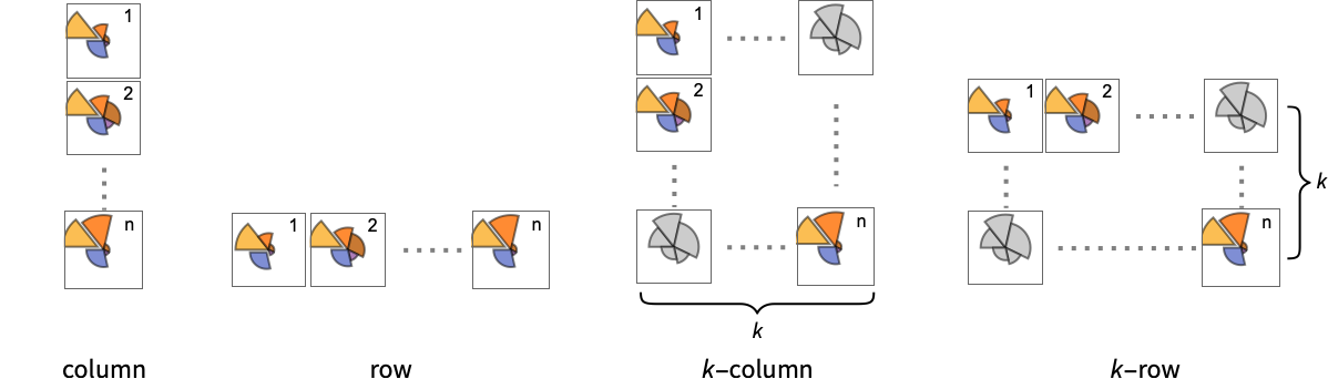
"Stacked" 累积每个数据集的数据
在不同面板中显示单个数据组的 ChartLayout 的可能设置包括：

	"Column"	在一列面板中分别使用不同扇区组
	"Row"	在一行面板中分别使用不同扇区组
	{"Column",k},{"Row",k}	使用 k 列或行
	{"Column",UpTo[k]},{"Row",UpTo[k]}	使用至多 k 列或行

ChartElementFunction 的参数是扇形区域 {{θ_min,θ_max},{r_min,r_max}}，值 {x_i,y_i} 和数据集的嵌套列表中每层的元数据 {m₁,m₂,…}.
ChartElementFunction 的内置列表可以从 ChartElementData["SectorChart"] 得到.
ColorFunction 的参数是 θ 和 r，θ 是扇形的角度，r 是半径.
SectorChart 中选项和其它结构的样式和其它设置按照 ChartStyle、ColorFunction、Style 和和其他包装和 ChartElementFunction，后面的设置会屏蔽之前的设置.

所有选项的列表

AlignmentPoint	Center	在图形内对齐的缺省点
AspectRatio	Automatic	高与宽的比
Axes	False	是否绘制轴
AxesLabel	None	坐标轴标签
AxesOrigin	Automatic	坐标轴原点
AxesStyle	{}	坐标轴样式指定
Background	None	绘图的背景色
BaselinePosition	Automatic	如何与环绕文本基线对齐
BaseStyle	{}	图形的基本样式指定
ChartBaseStyle	Automatic	扇形的整体样式
ChartElementFunction	Automatic	如何产生扇形的原图形
ChartLabels	None	数据元素和数据集的标签
ChartLayout	Automatic	使用的整体布局
ChartLegends	None	数据元素和数据集的图例
ChartStyle	Automatic	扇形的样式
ColorFunction	Automatic	如何着色扇形
ColorFunctionScaling	True	是否标准化参数到 ColorFunction
ContentSelectable	Automatic	是否允许进行内容选择
CoordinatesToolOptions	Automatic	坐标工具的详细行为
Epilog	{}	主图形之后执行的图形指令
FormatType	TraditionalForm	文本的缺省样式类型
Frame	False	是否在图形周围放置边框
FrameLabel	None	边框标签
FrameStyle	{}	边框的样式指定
FrameTicks	Automatic	边框刻度
FrameTicksStyle	{}	边框刻度的样式指定
GridLines	None	绘制的网格线
GridLinesStyle	{}	网格线的样式指定
ImageMargins	0.	图形周围的边幅
ImagePadding	All	为标签等额外填充内容
ImageSize	Automatic	图形的绝对尺寸
LabelingFunction	Automatic	如何标注扇形
LabelingSize	Automatic	标注和标签的最大尺寸
LabelStyle	{}	标签的样式指定
LegendAppearance	Automatic	图例的整体外观
Method	Automatic	使用图形方式的细节
PerformanceGoal	$PerformanceGoal	优化执行的方面
PlotLabel	None	图形的一个整体标签
PlotRange	Automatic	包含值的范围
PlotRangeClipping	False	是否在图形范围剪切
PlotRangePadding	Automatic	填充图形值范围的程度
PlotRegion	Automatic	填充的最后显示区域
PlotTheme	$PlotTheme	图表的整体主题
PolarAxes	False	是否绘制极轴
PolarAxesOrigin	Automatic	在哪里绘制极轴
PolarGridLines	None	极坐标网格线
PolarTicks	Automatic	极轴刻度
PreserveImageOptions	Automatic	当显示相同图形的新版本时，是否保存图形选项
Prolog	{}	主图形之前执行的图形指令
RotateLabel	True	是否在边框上旋转 y 标签
SectorOrigin	Automatic	初始角度和扇形弧度
SectorSpacing	Automatic	扇形间的间距
TargetUnits	Automatic	图表中显示的单位
Ticks	Automatic	坐标轴标记
TicksStyle	{}	坐标轴标记的样式指定

范例

打开所有单元关闭所有单元

基本范例 (5)

第二个分量表示弧度大小的扇图：

环扇形图：

多个数据集：

将多个数据组显示为一行扇区图表：

使用分类标签：

分类图例：

设置扇区样式：

范围 (38)

数据和布局 (13)

数据集中的元素分组：

数据集不需要有相同数量的元素：

在饼图中忽略非实数数据：

数据可能包括单位：

忽略 TimeSeries、EventSeries 和 TemporalData 中的时间戳：

相关性中的数值作为扇区的数值：

将键作为标签使用：

用键作为标注 (callout):

将键作为图例使用：

包装 (4)

在单个数据、数据集或一组数据集中用包装：

可以嵌套包装：

屏蔽缺省的工具提示：

用工具提示中的任何对象：

用 PopupWindow 进一步提供信息：

Button 可以用于触发任何行为：

样式和外观 (9)

对于扇形用明确的样式列表：

使用 ColorData 中任何梯度或索引颜色方案：

为图表设计的颜色方案：

使用主题控制整体外观：

ChartBaseStyle 可以对所有图表元素设置一个初始样式：

Style 可以用于屏蔽样式：

用内置的程序产生扇形：

用面板 ▶ 图表元素方案具体设置：

使用具有黑色背景和边框扇区的主题：

使用单色主题：

标签和图例 (12)

使用 Labeled 对扇区添加标签：

对标签放置，使用符号式位置：

对数据列，使用分类标签：

对数据列：

对两者：

使用 Placed 来控制标签位置，使用与 Labeled 中相同的位置:

用 Callout 为扇区添加标签：

改变标注的外观：

自动放置标注：

通过使用 LabelingFunction 添加数值标签：

根据数据生成标注：

对数据列，添加分类图例项目：

对于数据行：

使用 Legended 来添加额外的图例项目：

使用 Placed 来影响图例位置：

选项 (56)

ChartBaseStyle (5)

用 ChartBaseStyle 设置所有扇形的样式：

ChartBaseStyle 和 ChartStyle 连用：

ChartStyle 可能屏蔽 ChartBaseStyle 的设置：

ChartBaseStyle 和 Style 连用：

Style 可能屏蔽 ChartBaseStyle 的设置：

ChartBaseStyle 和 ColorFunction 连用：

ColorFunction 可能屏蔽 ChartBaseStyle 的设置：

ChartElementFunction (5)

获得 ChartElementFunction 内置的设置列表：

用面板 ▶ 图表元素方案具体设置：

用 ChartElementData 指定相同的图形渲染函数如上：

写入一个定制的 ChartElementFunction：

用输入传递的元数据，这里对数据制图：

ChartLabels (8)

缺省下标签被放置在中心：

数据中的 Labeled 包装将放置其它标签：

用 Placed 控制标签放置：

扇形外的位置：

标注位置：

基于相对一个扇形放置的坐标：

将所有标签放在第一个外面的角落并改变标签内的坐标：

用 Placed 的第三个参数控制格式化：

使用超链接标签：

缺省下标签和数据列相关：

标签和行或数据集相关：

同时标注行和列：

用 Placed 影响位置：

用 Callout 来把标签连接到扇区：

放置多个标签：

ChartLayout (4)

ChartLayout 按同心环分组：

用堆栈扇形：

堆栈布局可以显示多个数据集：

使用共用尺寸将每个扇区置于不同面板：

使用一行而非一列：

使用多列或多行：

将偏好设为满行或满列：

ChartLegends (4)

产生基于图表样式的图例：

用 Legended 增加其它图例项：

或指定单个图例项：

产生数据集的图例：

删除未使用的图例标签：

图例可以作用在多个维上：

用 Placed 控制图例的放置：

ChartStyle (6)

用 ChartStyle 设置扇形的样式：

给出一个样式列表：

使用 ColorData 的"Gradient"颜色：

用 ColorData 的"Indexed" 颜色：

循环使用样式：

每个数据列的样式：

每个数据行的样式：

数据行和数据列的样式：

若同时设置行和列的样式，最后的样式会屏蔽之前的样式：

Style 屏蔽 ChartStyle 的设置：

ColorFunction 屏蔽 ChartStyle 的设置：

ColorFunction (4)

按扇形角度着色：

用 ColorFunctionScaling->False，获得未调整的角度值：

按区域着色：

ColorFunction 屏蔽 ChartStyle 中的样式：

用 ColorFunction 组合不同样式效果：

ColorFunctionScaling (2)

用 ColorFunctionScaling->False 得到未调整的高度值：

按区域着色：

ImageSize (7)

使用有名称尺寸 Tiny、Small、Medium 和 Large：

指定绘图的宽度：

指定绘图的高：

允许宽和高在设定的最大值之内取值：

为图形指定宽度和高度，如有必要填充该空间：

使用宽度和高度的最大尺寸：

使用 ImageSizeFull 填充对象内的可用空间：

将图形尺寸指定为可用空间的一个比例：

LabelingFunction (8)

Tooltip 和 StatusArea 使用自动标签：

不使用标签：

用 Placed 控制标签放置：

在扇形外的符号位置：

标注标签的位置：

基于相对一个条放置的坐标：

用 Callout 自动放置标签：

控制标签的格式化：

用给出的图表标签，作为标签函数的参数：

LabelingSize (3)

文本标签以实际尺寸显示：

图像标签自动调整：

指定文本标签的最大尺寸：

指定图像标签的最大尺寸：

应用 (7)

产生一个扇形图：

产生一个矢量图：

产生一个圆列图：

点击扇形听取该国的名称，其人均国内生产总值和人口：

建立一个营养含量的雷达图：

可视化人均国内生产总值：

对每一个扇形加一个别致的 Tooltip 标签：

从 0° 到 360° 的 WeatherData 中的风向：

得到伊利诺伊州，香槟威拉德机场 (CMI) 的风向：

删除缺少的数据：

用 Sow 定义一个图表元素函数，来存储组距和频数数据：

创建一个风向的直方图，来存储组距和频数：

创建一个风向频数的极坐标直方图：

属性和关系 (4)

SectorChart 是 PieChart 的一般化：

使用 SectorChart3D 得到一个三维扇形图：

使用 RectangleChart 把成对数绘制成条状：

使用 ListPlot 和 ListLinePlot 从成对数产生线图：

巧妙范例 (3)

运用刻度增加图表细节：

运用网格线增加图表细节：

例如以下图表：

顶部

		"Grouped"	分离每个数据集的数据
		"Stacked"	累积每个数据集的数据