



SolveValues
SolveValues[expr,vars]
给出由系统 expr 的解确定的 vars 的值.
SolveValues[expr,vars,dom]
更多信息和选项
- 系统 expr 可以是以下内容的任何逻辑组合:
-
lhs==rhs 等式 lhs!=rhs 不等式 lhs>rhs 或 lhs>=rhs 不等式 expr∈dom 定义域规范 {x,y,…}∈reg 区域规范 ForAll[x,cond,expr] 通用量词 Exists[x,cond,expr] 存在量词 - SolveValues[{expr1,expr2,…},vars] 等价于 SolveValues[expr1&&expr2&&…,vars].
- 如果指定了单个变量,则结果是使 expr 为 True 的变量值列表.
- 如果指定了变量列表,则结果是使 expr 为 True 的变量值列表的列表.
- 当指定单个变量且方程特根的多重性大于 1 时,SolveValues 会提供相应解的多个副本.
- SolveValues[expr,vars] 默认假设不等式中以代数形式出现的数量是实数,而所有其他量都是复数.
- SolveValues[expr,vars,dom] 限定所有变量和参数均属于定义域 dom.
- 如果 dom 为 Reals 或诸如 Integers 或 Rationals 等子集, 则所有常量和函数值也都被限定为实数.
- SolveValues[expr&&vars∈Reals,vars,Complexes] 求解变量的实数值,但函数值可以是复数.
- SolveValues[expr,vars,Integers] 在整数上求解丢番图方程.
- SolveValues[…,x∈reg,Reals] 将 x 约束在区域 reg 中. 可以使用 Indexed[x,i] 引用 x 的不同坐标.
- 在 expr 中无 vars 的代数变量被视为独立参数.
- SolveValues 主要处理线性和多项式方程.
- 当 expr 仅涉及实数或复数域上的多项式方程式和不等式时,SolveValues 原则上始终可以直接求解 vars.
- 当 expr 涉及超越条件或整数域时,SolveValues 通常会在其结果中引入其他参数.
- SolveValues 可以给出所有线性方程和不等式的整数解的显式表示形式,并且可以求解文献中描述的大部分丢番图方程.
- 当 expr 仅涉及实数域或复数域上的多项式条件时,SolveValues[expr,vars] 将始终能够消除量词.
- SolveValues 仅提供通解. 仅在连续参数满足方程式时有效的解将被删除. 其他仅在一定条件上有效的解则表示为 ConditionalExpression 对象.
- 在 ConditionalExpression 解中包括的条件可能涉及不等式、Element 语句、非连续参数上的方程和不等式及具有全维解的方程. 连续参数和变量上的不等式和 NotElement 条件将被舍弃.
- SolveValues 可能使用非等价变换来求超越方程的解,因此可能找不到某些解,并且可能无法为所得到的解的有效性建立确切条件. 如果发生这种情况,将发出错误消息.
- SolveValues 使用特殊的有效技术来处理具有近似数值系数的稀疏线性方程组.
- 可以给出以下选项:
-
Assumptions $Assumptions 对参数的假设 Cubics Automatic 是否使用显式根式来求解所有三次方程 GeneratedParameters C 如何命名生成的参数 InverseFunctions Automatic 是否使用符号式反函数 MaxExtraConditions 0 在连续参数上所允许的额外等式条件数 MaxRoots Infinity 返回的根的最大数目 Method Automatic 应该使用什么方法 Modulus 0 整数假设的模数 Quartics Automatic 是否使用显式根式来解决所有四次方程 VerifySolutions Automatic 是否验证使用非等价变换获得的解 WorkingPrecision Infinity 计算中使用的精度 - 使用 MaxExtraConditions->Automatic,仅包含需要在连续参数上具有最少数量等式条件的解.
- 使用 MaxExtraConditions->All,将给出在参数上需要任意条件的解,并且包括所有条件.
- 使用 MaxExtraConditions->k,仅包括在连续参数上最多需要 k 个等式条件的解.
- 使用 Method->Reduce,SolveValues 仅使用等效转换并找到所有解.
- SolveValues[eqns,…,Modulus->m] 在整数模 m 上求解方程. 使用 Modulus->Automatic,SolveValues 将尝试找到使方程有解的最大模数.
范例
打开所有单元 关闭所有单元基本范例 (5)
SolveValues[x ^ 2 + a x + 1 == 0, x]

SolveValues[a x + y == 7 && b x - y == 1, {x, y}]SolveValues[(x ^ 2 + 2)(x ^ 2 - 2) == 0, x, Reals]SolveValues[x ^ 2 + 2y ^ 3 == 3681 && x > 0 && y > 0, {x, y}, Integers]SolveValues[{x, y}∈InfiniteLine[{{0, 0}, {2, 1}}] && {x, y}∈Circle[], {x, y}]Graphics[{{Blue, InfiniteLine[{{0, 0}, {2, 1}}], Circle[]}, {PointSize[Large], Red, Point[%]}}]范围 (87)
基本用法 (7)
sol = SolveValues[x ^ 2 + y ^ 2 == 2 && x - y == 1, {x, y}]x ^ 2 + y ^ 2 == 2 && x - y == 1 /. Thread[{x, y} -> #]& /@ %如果无解,SolveValues 将返回空列表:
SolveValues[x == 1 && x == 2, x]SolveValues[x + y == 1, {x, y}]
SolveValues[(x ^ 4 - 1)(x ^ 4 - 4) == 0, x, Complexes]SolveValues[(x ^ 4 - 1)(x ^ 4 - 4) == 0, x, Reals]SolveValues[(x ^ 4 - 1)(x ^ 4 - 4) == 0, x, Integers]sol = SolveValues[x ^ 2 + y ^ 2 == 1 && x + y == a, {x, y}]Plot[Evaluate[Re[#[[2]]]& /@ sol], {a, 0, 2}]sol = SolveValues[x ^ 2 + a x + b == 0, x, Reals]使用 Normal 删除条件:
Normal[sol]sol = SolveValues[x ^ 2 - 2y ^ 2 == 1 && x > 0 && y > 0, {x, y}, Integers]First[sol] /. Table[{C[1] -> i}, {i, 10}]//Simplify单变量复数方程 (16)
SolveValues[x ^ 4 - x ^ 2 - 5 == 0, x]要使用通用公式求解三次方程式,需设置 CubicsTrue:
SolveValues[x ^ 3 - 2x ^ 2 + 5x + 7 == 0, x, Cubics -> True]默认情况下,SolveValues 使用 Root 对象表示一般三次方程的解:
SolveValues[x ^ 3 - 2x ^ 2 + 5x + 7 == 0, x]SolveValues[x ^ 5 - 2x + 17 == 0, x]SolveValues[(x ^ 2 - 1)(x ^ 4 - 1) == 0, x]SolveValues[x ^ 1234567 + 9x ^ 2 + 7x - 1 == 0, x, MaxRoots -> 5]SolveValues[a x ^ 2 + b x + c == 0, x]SolveValues[a x ^ 5 + b x + c == 0, x]SolveValues[Sqrt[x] + 3x ^ (1 / 3) == 5, x]SolveValues[Sin[x] == 1 / 3, x]SolveValues[(x ^ 5 - 1) ^ x == 0, x]SolveValues[x ^ (2a) + 2x ^ a + 1 == 0, x]
SolveValues[ArcTan[1 / Sqrt[1 + x ^ 2], x / Sqrt[1 + x ^ 2]] == a, x]
SolveValues 无法在这里找到所有解:
SolveValues[5 == x * 2 ^ (x ^ 2), x]
SolveValues[5 == x * 2 ^ (x ^ 2), x, MaxRoots -> 3]SolveValues[Sin[E ^ x] - Cos[2 x] == 1 && -1 ≤ Re[x] ≤ 1 && -1 ≤ Im[x] ≤ 1, x]SolveValues[Gamma[x] - Log[x] == I / 2 && Abs[x - 2] < 3 / 2, x]
这里 SolveValues 找到了一些解,但无法证明没有其他解:
SolveValues[x == E ^ (1 / x) && Abs[x] < 5, x]
SolveValues[Cos[Exp[x]] == 3 Exp[-x] + 1 && 0 ≤ Re[x] ≤ 1, x]SolveValues[Sin[FresnelS[x] + BesselJ[3, x ^ 2 - 1]] == 2 ^ Cos[x] - 3, x, MaxRoots -> 5]SolveValues[f[x] ^ 3 + 2f[x] - 3 == 0, x]
SolveValues[{Re[x] + Im[x]^2 == 1, Re[x] - Im[x] == -1}, x]SolveValues[{Abs[x] == 1, Arg[x] == π / 4}, x]多变量复方程组 (12)
SolveValues[{x + 2y + 3z == 4, 3x + 4y + 5z == 6, 7x + 7y + 8z == 9}, {x, y, z}]SolveValues[a x + b y + c z == d && 3x + 4y + 5z == 6 && 7x + 7y + 8z == 9, {x, y, z}]SolveValues[x + 2y + 3z == 4 && 3x + 4y + 5z == 6 && 6x + 7y + 8z == 9, {x, y, z}]
SolveValues[x + 2y + 3z == 4 && 3x + 4y + 5z == 6 && 6x + 7y + 8z == 0, {x, y, z}]SolveValues[x ^ 2 + y ^ 2 == 1 && x + 2y == 3, {x, y}]SolveValues[x ^ 10000 == y ^ 2 + 3y + 2 && y ^ 10000 == z ^ 2 + 3z + 2 && z ^ 10000 == x ^ 2 + 3x + 2, {x, y, z}, MaxRoots -> 5]SolveValues[a x ^ 2 + b y ^ 2 == c && x + 2y == 3, {x, y}]SolveValues[Sqrt[x y] == Sqrt[x + y] && Sqrt[x] - y ^ (1 / 3) == 1, {x, y}]
SolveValues[Sin[x + y] == 1 && Log[x - y] == 1 / 2, {x, y}]SolveValues[3 ^ x ^ 2 == 7 && x ^ 2 - y ^ 3 == 4, {x, y}]
SolveValues[Sin[x + y] == x y + 1 && Cos[x - y] == AiryAi[x y] + 2, {x, y}, MaxRoots -> 3]SolveValues[FresnelS[x - y] - AiryAi[x] + y == (3 + I) / 2 && CosIntegral[x] y - Sin[x y] == -5(1 - I) / 4 && 1 ≤ Re[x] ≤ 2 && 0 ≤ Im[x] ≤ 1 && 1 ≤ Re[y] ≤ 2 && 0 ≤ Im[y] ≤ 1, {x, y}]SolveValues[{Re[x^2] + Im[y] == 1, x^2 - y^2 == 0, Im[x^3] - Im[y]^2 == 2}, {x, y}]单变量实数方程 (13)
SolveValues[x ^ 5 - 2x + 1 == 0, x, Reals]SolveValues[(x ^ 2 - 1)(x ^ 4 - 1) == 0, x, Reals]SolveValues[x ^ 3 + a x + a ^ 2 == 0, x, Reals]SolveValues[Sqrt[x] + 3x ^ (1 / 3) == 5, x, Reals]SolveValues[Abs[x] ^ 2 - x + UnitStep[x] == 9, x, Reals]SolveValues[E ^ x - x == 7, x, Reals]SolveValues[ 27^2x - 1^(1/(x)) == Sqrt[9^2x - 1], x, Reals]SolveValues[JacobiSN[x, y] == 1, x, Reals]SolveValues[AiryBi[1 - x ^ 2] == 0 && 2 < x < 3, x, Reals]SolveValues[900 < AiryAiZero[2t + 1] ^ 2 < 1000, t, Reals]SolveValues[E ^ (2E ^ x) - Log[x ^ 2 + 1] - 20x == 11, x, Reals]SolveValues[x ^ 1000000 - 2x ^ 777777 + 3x ^ 12345 + 9x ^ 67 - 10 == 0, x, Reals]SolveValues[2x ^ (123451 / 67890) - x ^ 2 + 4Sqrt[x] - 4x - 9 / 8 == 0, x, Reals]SolveValues[x ^ Pi - x ^ x ^ Sqrt[2] - Sqrt[3]x + 2 ^ (1 / 3) == 0, x, Reals]SolveValues[E ^ (2x) + x ^ 4 + 4(x ^ 2 + 1) == (2x ^ 2 + 4)E ^ x, x, Reals]SolveValues[10Sin[Tan[E ^ -x ^ 2]] - x == 3, x, Reals]SolveValues[2Sin[Exp[x]] - Cos[Pi x] == 3 / 2 && -1 < x < 1, x, Reals]SolveValues[Cos[x] - BesselJ[5, x] == 1 / 2 && 0 ≤ x ≤ 10, x]
SolveValues[Exp[Sin[x]] - Sin[3 Cos[x]] == 0, x, Reals]多变量实数方程组和不等式组 (10)
SolveValues[2 x + 3y - 5z == 1 && 3x - 4y + 7z == 3, {y, z}, Reals]SolveValues[x y == z ^ 2 - x && x y z == 2 && x ^ 2 + y ^ 2 + z ^ 2 ≤ 5, {y, z}, Reals]SolveValues[Exists[x, x ^ 2 + a x + b == 0 && 2 x + a == 0], a, Reals]SolveValues[ForAll[x, Exists[y, a x ^ 2 + b y ^ 2 - 3y == 1 && y < 0 && a y - y == b + 1]], {a, b}, Reals]SolveValues[Sqrt[x + 2y] - 3x + 4y ≥ 5 && x + y ^ (1 / 3) == 1, y, Reals]SolveValues[Max[x, y] == Min[y ^ 2 - x, x] + y && z + UnitStep[x - y] == 1, {y, z}, Reals]SolveValues[Sin[x + y] == 1 / 2 && E ^ x - y ≤ 1, y, Reals]SolveValues[ 3^x - 2^2y == 77 && Sqrt[3^x] - 2^y == 7, {x, y}, Reals]SolveValues[E ^ x y ^ 3 + Log[x]y == 1 && x y + E ^ x / x ≥ 2, y, Reals]SolveValues[Exists[a, a x ^ 2 + Sinh[x ^ 2 + 1]a ^ 2 == 1 && x ^ 2 - a ^ 2 == 1], x, Reals]SolveValues[Sin[x - Cos[x]] y ^ 3 - x == 1 && x ^ 2 + y ^ 2 ≤ 1, y, Reals]SolveValues[Exists[y, y ^ 3 - Cos[x] y + 2 x ^ 2 Sin[x ^ 2 - 1] == 0 && x ^ 2 + y ^ 2 == 2], x, Reals]SolveValues[y ^ 3 - BesselJ[2, x + 2] y - y - 3 x == -2 && y < 0 && x ^ 2 < 2, y, Reals]
SolveValues[Exists[y, y ^ 4 - Gamma[x + 2] y - y - 3 ArcSin[x / 3] == 1 && x ^ 2 + y ^ 3 == 1 && 0 < x < 2], x, Reals]
SolveValues[Gamma[x + y + 1] - Sin[x y] == 1 && Erf[x ^ 2 - y] - E ^ y - x + 4 == 0 && 0 < x < 3 && 0 < y < 3, {x, y}, Reals]丢番图方程 (11)
SolveValues[2 x + 3y - 5z == 1 && 3x - 4y + 7z == 3, {x, y, z}, Integers]SolveValues[2 x + 3y == 4 && 3x - 4y ≤ 5 && x - 2y > -21, {x, y}, Integers]SolveValues[x ^ 12345 - 2x ^ 777 + 1 == 0, x, Integers]SolveValues[x ^ 2 + x y + y ^ 2 == 109, {x, y}, Integers]SolveValues[x ^ 2 - 3y ^ 2 == 22 && x > 0 && y > 0, {x, y}, Integers]SolveValues[x ^ 2 - 6 x y + 9y ^ 2 - x + 2y == 1, {x, y}, Integers]SolveValues[x ^ 3 - 2x ^ 2 y + y ^ 3 == 2, {x, y}, Integers]SolveValues[x ^ 2 + 4y ^ 2 + 9z ^ 2 + 16t ^ 2 == 354 && x > 0 && y > 0 && z > 0 && t > 0, {x, y, z, t}, Integers]SolveValues[x ^ 2 + y ^ 2 == z ^ 2, {x, y, z}, Integers]SolveValues[x ^ 4 + y ^ 4 + z ^ 4 ≤ 500 && x + y ^ 2 + z ^ 3 == 32, {x, y, z}, Integers]SolveValues[2x ^ 7 + 8y ^ 15 + 14 x y z == 3, {x, y, z}, Integers]SolveValues[Exp[y ^ 2] < x && Abs[x] < 5 && Abs[y] < 5, {x, y}, Integers]SolveValues[Exp[x ^ 2 - 5y ^ 2 + 1] + x ^ 2 - 5y ^ 2 == 0 && x > 0 && y > 0, {x, y}, Integers]SolveValues[Mod[x ^ 2 + y ^ 2, 2] == 1 && Mod[x - 2y, 3] == 2, {x, y}, Integers]模方程 (4)
SolveValues[2 x + 3y - 5z == 1 && 3x - 4y + 7z == 3 && 2x - 10y + 3z == 5, {x, y, z}, Modulus -> 12]SolveValues[2 x + 3y - 5z == 1 && 3x - 4y + 7z == 3, {x, y, z}, Modulus -> 12]
SolveValues[x ^ 3 - 2x + 1 == 0, x, Modulus -> 5]SolveValues[x ^ 2 + y ^ 3 == 1 && x + 2y ^ 2 == 4, {x, y}, Modulus -> 7]SolveValues[x ^ 2 + y ^ 3 == z && x + 2y == 3z + 1 && x y z ≠ 0, {x, y, z}, Modulus -> 7]SolveValues[ForAll[x, Exists[y, a x ^ 2 + b y ^ 2 - 3y == 1 && y ≠ 0]], {a, b}, Modulus -> 3]有限域上的方程 (3)
ℱ = FiniteField[53, 4];
SolveValues[x ^ 5 + ℱ[123]x == ℱ[234], x]SolveValues[x ^ 7 + 2 x + 3 == 0, x, ℱ]ℱ = FiniteField[71, 2];
SolveValues[ℱ[123]x + ℱ[234]y == ℱ[345] && ℱ[321]x + ℱ[432]y == ℱ[543], {x, y}]SolveValues[ℱ[1234]x + ℱ[2345]y + ℱ[3456]z == ℱ[4567] && ℱ[1]x + ℱ[2]y + ℱ[3]z == ℱ[4], {y, z}]ℱ = FiniteField[7, 5];
SolveValues[x ^ 2 + y ^ 2 == 3 && x ^ 5 + y ^ 5 == 5, {x, y}, ℱ]SolveValues[ℱ[123]x ^ 2 + ℱ[234]y ^ 3 + ℱ[345]z ^ 4 == ℱ[456] && ℱ[21]x + ℱ[32]y ^ 2 + ℱ[43]z ^ 3 == ℱ[54] && x y z == ℱ[1], {x, y, z}]具有混合变量域的系统 (2)
具有几何区域约束的系统 (9)
Subscript[ℛ, 1] = Circle[];
Subscript[ℛ, 2] = Line[{{-2, 1}, {1, -2}}];SolveValues[{x, y}∈Subscript[ℛ, 1] && {x, y}∈Subscript[ℛ, 2], {x, y}]Graphics[{{Blue, Subscript[ℛ, 1], Subscript[ℛ, 2]}, {Red, Point[%]}}]Subscript[ℛ, 1] = Sphere[];
Subscript[ℛ, 2] = InfinitePlane[{{0, 0, 0}, {0, 1, 0}, {1, 0, 1}}];SolveValues[2 x y == z^2 && {x, y, z}∈Subscript[ℛ, 1] && {x, y, z}∈Subscript[ℛ, 2], {x, y, z}, Reals]Show[{ContourPlot3D[2 x y == z^2, {x, -1.2, 1.2}, {y, -1.2, 1.2}, {z, -1.2, 1.2}, Mesh -> None, ContourStyle -> Opacity[0.5]], Graphics3D[{{Opacity[0.5], Green, Subscript[ℛ, 1]}, {Opacity[0.5], Yellow, Subscript[ℛ, 2]}, {PointSize[Large], Red, Point[%]}}]}]ℛ = Cone[{{0, 0, 0}, {1, 2, 3}}, 4];SolveValues[Subscript[∃, z](x^2 + y^2 == z^2 && x + y == z - 1 && {x, y, z}∈ℛ), y, Reals]ℛ = ImplicitRegion[a + 2 b - 3 c ≥ 1 && a b c == 7, {a, b, c}];SolveValues[y^2 + x z == 1 && {x, y, z}∈ℛ, {y, z}, Reals]ℛ = ParametricRegion[{s + t, s - t, s t}, {s, t}];SolveValues[x y == z && x + 2 y + 3 z == 1 && {x, y, z}∈ℛ, {x, y, z}, Reals]Subscript[ℛ, 1] = Disk[{0, 0}, 2];
Subscript[ℛ, 2] = Circle[{1, 1}, 2];
Subscript[ℛ, 3] = RegionIntersection[Subscript[ℛ, 1], Subscript[ℛ, 2]];SolveValues[x^2 == x y + 1 && {x, y}∈Subscript[ℛ, 3], {x, y}, Reals]Show[{ContourPlot[x^2 == x y + 1, {x, -2, 3}, {y, -2, 3}], Graphics[{{Opacity[0.5], Yellow, Subscript[ℛ, 1]}, {Green, Subscript[ℛ, 2]}, {Red, Point[%]}}]}]ℛ = RegionProduct[Circle[], Circle[]];SolveValues[Subscript[∃, {a, b}](4 x y a b == 1 && {x, a, y, b}∈ℛ), {x, y}, Reals]Subscript[ℛ, 1] = InfiniteLine[{{2, 0}, {0, t}}];
Subscript[ℛ, 2] = Circle[];
SolveValues[{x, y}∈Subscript[ℛ, 1] && {x, y}∈Subscript[ℛ, 2], {x, y}, Reals]


ℛ = RegionIntersection[Circle[], Line[{{-2, -1}, {1, 2}}]];SolveValues[x∈ℛ, x]

ℛ = Sphere[];SolveValues[x.{1, 2, 3} == 0 && x.{-3, -2, -1} == 0 && x∈ℛ, x]选项 (26)
Assumptions (4)
使用 Assumptions 指定关于参数的条件:
SolveValues[x ^ 2 == a, x, Reals, Assumptions -> a > 0]SolveValues[x ^ 2 == a, x, Reals, Assumptions -> a < 0]SolveValues[s == (2t) / (1 + t ^ 2) && c == (1 - t ^ 2) / (1 + t ^ 2), t]SolveValues[s == (2t) / (1 + t ^ 2) && c == (1 - t ^ 2) / (1 + t ^ 2), t, Assumptions -> s ^ 2 + c ^ 2 == 1]SolveValues[2 ^ x == 8, x, Assumptions -> x > 0]不使用 Assumptions 的等效语句:
SolveValues[2 ^ x == 8 && x > 0, x]SolveValues[a x ^ 2 + b x + c == 0, x, Assumptions -> Element[a, Integers]]
Cubics (3)
默认情况下,仅当存在符号参数时,SolveValues 才使用带根式的三次方程的通用求根公式求解:
SolveValues[x ^ 3 + a x ^ 2 + 2 x + 3 == 0, x]对于具有数字系数的多项式,SolveValues 不使用求根公式:
SolveValues[x ^ 3 + 2 x ^ 2 + 3 x + 4 == 0, x]使用 Cubics->False,SolveValues 从不使用求根公式:
SolveValues[x ^ 3 + a x ^ 2 + 2 x + 3 == 0, x, Cubics -> False]使用 Cubics->True,SolveValues 始终使用求根公式:
SolveValues[x ^ 3 + 2 x ^ 2 + 3 x + 4 == 0, x, Cubics -> True]GeneratedParameters (1)
SolveValues 可能会引入新的参数来表示解:
SolveValues[x ^ 2 - 3y ^ 2 == 1 && x > 0 && y > 0, {x, y}, Integers]使用 GeneratedParameters 控制参数如何生成:
SolveValues[x ^ 2 - 3y ^ 2 == 1 && x > 0 && y > 0, {x, y}, Integers, GeneratedParameters -> (Subscript[k, #]&)]InverseFunctions (3)
默认情况下,SolveValues 使用反函数,但显示警告消息:
SolveValues[f[x] == 0, x]
SolveValues[x + E ^ x == 1, x]
对于具有 NumericFunction 属性的符号,不使用符号反函数:
SolveValues[Gamma[x] == a, x]
使用 InverseFunctions->True,SolveValues 不显示反函数警告消息:
SolveValues[f[x] == 0, x, InverseFunctions -> True]SolveValues[x + E ^ x == 1, x, InverseFunctions -> True]SolveValues[Gamma[x] == a, x, InverseFunctions -> True]使用 InverseFunctions->False,SolveValues 不使用反函数:
SolveValues[f[x] == 0, x, InverseFunctions -> False]
SolveValues[x ^ 2 + 1 == 0, x, InverseFunctions -> False]在这里,使用了基于 Reduce 的方法,因为它不需要使用反函数:
SolveValues[x + E ^ x == 1, x, InverseFunctions -> False]MaxExtraConditions (4)
SolveValues[a == 0 && x == 0, x]SolveValues[a == 0 && x == 0, x, Integers]默认设置 MaxExtraConditions->0 不给出需要条件的解:
SolveValues[(x - a)(x - b) == 0 && (x - c)(x - d) == 0 && (x - a)(x - e) == 0, x]SolveValues[(x - a)(x - b) == 0 && (x - c)(x - d) == 0 && (x - a)(x - e) == 0, x, MaxExtraConditions -> 0]MaxExtraConditions->1 给出需要最多一个参数方程的解:
SolveValues[(x - a)(x - b) == 0 && (x - c)(x - d) == 0 && (x - a)(x - e) == 0, x, MaxExtraConditions -> 1]MaxExtraConditions->2 给出最多需要两个参数方程的解:
SolveValues[(x - a)(x - b) == 0 && (x - c)(x - d) == 0 && (x - a)(x - e) == 0, x, MaxExtraConditions -> 2]SolveValues[(x - a)(x - b) == 0 && (x - c)(x - d) == 0 && (x - a)(x - e) == 0, x, MaxExtraConditions -> Automatic]SolveValues[(x - a)(x - b) == 0 && (x - c)(x - d) == 0 && (x - a)(x - e) == 0, x, MaxExtraConditions -> All]默认情况下,SolveValues 删除连续参数上的不等式条件:
Solve[a x == 1, x]使用 MaxExtraConditions->All,SolveValues 包括所有条件:
SolveValues[a x == 1, x, MaxExtraConditions -> All]MaxRoots (4)


SolveValues[x ^ 12345 + x + 1 == 0, x, MaxRoots -> 3]

SolveValues[x ^ 1000 == y ^ 3 + 1 && y ^ 1000 == z ^ 3 + 1 && z ^ 1000 == x ^ 3 + 1, {x, y, z}, MaxRoots -> 3]
SolveValues[Sin[x + y] == 2x + 3y + 1 && AiryAi[x ^ 2 - y] == y ^ 2 - 1, {x, y}, MaxRoots -> 5]SolveValues[x ^ 4 == a, x, MaxRoots -> 3]
Method (1)
默认情况下,SolveValues 使用反函数来求解非多项式复数方程:
SolveValues[x E ^ x == 1 / 2, x]
设置 Method->Reduce,SolveValues 将使用 Reduce 找到完整的解集:
SolveValues[x E ^ x == 1 / 2, x, Method -> Reduce]Modulus (1)
Quartics (3)
默认情况下,仅当存在符号参数时,SolveValues 才使用带根式的四次方程的通用求根公式求解:
SolveValues[x ^ 4 + a x ^ 2 + 2 x + 3 == 0, x][[1]]对于具有数字系数的多项式,SolveValues 不使用求根公式:
SolveValues[x ^ 4 + 2 x ^ 2 + 3 x + 4 == 0, x]使用 Quartics->False,SolveValues 从不使用求根公式:
SolveValues[x ^ 4 + a x ^ 2 + 2 x + 3 == 0, x, Quartics -> False]使用 Quartics->True,SolveValues 始终使用求根公式:
SolveValues[x ^ 4 + 2 x ^ 2 + 3 x + 4 == 0, x, Quartics -> True][[1]]VerifySolutions (1)
SolveValues 验证使用非等效转换获得的解:
eqns = Sqrt[x + Sqrt[x]] == 2 && y ^ 9 - y - 2 x ^ (1 / 7) == 3;
(sol1 = SolveValues[eqns, {x, y}]);//Timing
使用 VerifySolutions->False,SolveValues 不验证解:
(sol2 = SolveValues[eqns, {x, y}, VerifySolutions -> False]);//Timing使用 VerifySolutions->False 返回的某些解不正确:
Length /@ {sol1, sol2}(sol3 = Select[sol2, TrueQ[eqns /. Thread[{x, y} -> N[#, 20]]]&]);//Timingsol3 === sol1WorkingPrecision (1)
默认情况下,SolveValues 得到方程的精确解:
SeedRandom[0];
mat = Table[RandomInteger[{-10 ^ 100, 10 ^ 100}], {200}, {200}];
b = Table[RandomInteger[{-10 ^ 100, 10 ^ 100}], {200}];
vars = x /@ Range[200];
(sol = SolveValues[Thread[mat.vars == b], vars]);//Timing(sol1 = SolveValues[Thread[mat.vars == b], vars, WorkingPrecision -> 100]);//TimingMax[Abs[sol - sol1]](sol2 = SolveValues[Thread[mat.vars == b], vars, WorkingPrecision -> MachinePrecision]);//TimingMax[Abs[sol - sol2]]应用 (7)
SolveValues[a x ^ 2 + b x + c == 0, x]pts = SolveValues[x ^ 2 + y ^ 2 == 1 && y - 2x ^ 2 + 3 / 2 == 0, {x, y}]Show[{ContourPlot[{x ^ 2 + y ^ 2 == 1, y - 2x ^ 2 + 3 / 2 == 0}, {x, -1.5, 1.5}, {y, -1.5, 1.5}], Graphics[{Red, PointSize[Medium], Point[pts]}]}]f[x_] := x ^ 4 + a x ^ 3 + b x ^ 2 + c x + d一种方法是使用 Subresultants:
SolveValues[Thread[Drop[Subresultants[f[x], D[f[x], x], x], -1] == 0], {b, c, d}]SolveValues[Exists[x, f[x] == 0, ForAll[y, f[y] == 0, x == y]], {b, c, d}]curve = x ^ 2 + y ^ 2 + z ^ 2 == 1 && x ^ 3 + x y ^ 2 == z ^ 2;sol = SolveValues[curve, {y, z}, Reals]cond = Union[#[[2]]& /@ Cases[sol, _ConditionalExpression, Infinity]]{l, u} = N[{cond[[1, 1]], cond[[1, 5]]}]ParametricPlot3D[Prepend[#, x]& /@ sol, {x, l, u}]proj = SolveValues[Exists[z, curve], y, Reals]ParametricPlot[{x, #}& /@ proj, {x, l, u}]SolveValues[x ^ 2 + y ^ 2 == 5 ^ 2 && y > x > 0, {x, y}, Integers]Table[SolveValues[x ^ 2 + y ^ 2 == z ^ 2 && y > x > 0, {x, y}, Integers], {z, 30}]求如何使用 10 美分、23 美分和 37 美分的邮票支付 2.27 美元的邮资:
SolveValues[a 10 + b 23 + c 37 == 227 && a >= 0 && b >= 0 && c >= 0, {a, b, c}, Integers]使用 IntegerPartitions 可以完成相同的任务:
IntegerPartitions[227, All, {37, 23, 10}]rts = SolveValues[Sin[x ^ 3] - x ^ 5 == 1, x, MaxRoots -> 200];ComplexPlot[Sin[x ^ 3] - x ^ 5 - 1, {x, -7.5 - 7.5I, 7.5 + 7.5I}, ...]属性和关系 (15)
eqns = {x ^ 2 + y ^ 2 == 1 && 2x + 3y == 4};SolveValues[eqns, {x, y}]eqns /. Thread[{x, y} -> #]& /@ %对于一元方程,SolveValues 根据其多重性重复求解:
SolveValues[(x - 1) ^ 2(x - 2) ^ 3 == 0, x]代数方程的解通常以 Root 对象的形式给出:
SolveValues[x ^ 5 - 2x + 7 == 0, x]N[%, 20]Root 对象可能涉及参数:
SolveValues[x ^ 5 + a x + 1 == 0, x]Series[%[[1]], {a, 0, 10}]x ^ 5 + a x + 1 /. x -> %SolveValues 给出解的值:
SolveValues[x ^ 4 == 4, x]Solve 根据替换规则表示解:
Solve[x ^ 4 == 4, x]Reduce 用方程和不等式的布尔组合表示解:
Reduce[x ^ 4 == 4, x]SolveValues 使用快速试探法求解超越方程,但可能给出不完整的解:
SolveValues[x - E ^ x == 1, x]
SolveValues[x Log[x] == a, x]
Reduce 使用的方法通常较慢,但会找到全部解并给出所有必要条件:
Reduce[x - E ^ x == 1, x]Reduce[x Log[x] == a, x]使用 FindInstance 求解的实例:
FindInstance[x ^ 2 + y ^ 2 + z ^ 2 == 1 && 2x y == z ^ 3, {x, y, z}]像 Reduce 一样,可以给 FindInstance 提供不等式和定义域规范:
FindInstance[x ^ 2 - 3y ^ 2 == 1 && 0 < x < 10 ^ 10, {x, y}, Integers, 3]使用 DSolve 求解微分方程:
DSolve[y''[x] == -y[x], y[x], x]DSolve[{y''[x] == -y[x], y[0] == 0, y'[0] == 1}, y[x], x]使用 RSolve 求解递归方程:
RSolve[f[n + 1] == n f[n], f[n], n]RSolve[{f[n + 1] == n + f[n], f[0] == 0}, f[n], n]SolveAlways 给出复方程始终为真的参数的值:
SolveAlways[(a - 2b + 1)x ^ 2 + (a - b ^ 2 - c)x == a ^ 2 - b + 3c - 1, x]相同的问题可以使用 ForAll 来表示,并使用 SolveValues、Solve 或 Reduce 来求解:
SolveValues[ForAll[x, (a - 2b + 1)x ^ 2 + (a - b ^ 2 - c)x == a ^ 2 - b + 3c - 1], {a, b, c}]Solve[ForAll[x, (a - 2b + 1)x ^ 2 + (a - b ^ 2 - c)x == a ^ 2 - b + 3c - 1], {a, b, c}]Reduce[ForAll[x, (a - 2b + 1)x ^ 2 + (a - b ^ 2 - c)x == a ^ 2 - b + 3c - 1], {a, b, c}]Resolve 消除量词,可能并不会求解得到的无量词系统:
Resolve[Exists[x, x ^ 2 + y ^ 2 + z ^ 2 == 1 && x y > z ^ 3], Reals]Resolve[ForAll[{x, y}, a x ^ 2 + b x + c == 0 && a y ^ 2 + b y + c == 0, x == y]]Eliminate 消除复方程组中的变量:
Eliminate[x ^ 2 + y ^ 2 + z ^ 2 == 1 && x z == y ^ 3, x]这里使用 Resolve 求解相同的问题:
Resolve[Exists[x, x ^ 2 + y ^ 2 + z ^ 2 == 1 && x z == y ^ 3]]Reduce、Solve 和 SolveValues 还可求解所得出的方程:
Reduce[Exists[x, x ^ 2 + y ^ 2 + z ^ 2 == 1 && x z == y ^ 3], {y, z}]Solve[Exists[x, x ^ 2 + y ^ 2 + z ^ 2 == 1 && x z == y ^ 3], z]SolveValues[Exists[x, x ^ 2 + y ^ 2 + z ^ 2 == 1 && x z == y ^ 3], z]


SolveValues[x ^ 3 + x + 1 == y, x, Reals]SolveValues[x ^ 2 + x + 1 == y, x, Reals]使用 FunctionBijective 检验函数是否是双射的:
FunctionBijective[x ^ 3 + x + 1, x]FunctionBijective[x ^ 2 + x + 1, x]使用 FunctionAnalytic 检验一个函数是否是解析的:
f = Sin[3x ^ 3] - 2x + 1;FunctionAnalytic[f, x, Complexes]SolveValues[f == 0 && Abs[x] ≤ 1, x]ComplexPlot[f, {x, -1 - I, 1 + I}, RegionFunction -> (Abs[#] ≤ 1&), Epilog -> {PointSize[Medium], Blue, Point[ReIm[%]]}]SolveValues 找到满足方程 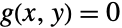 的
 的显式函数:
g = y ^ 3 - x y ^ 2 + 2x ^ 2y - x + 1;y1 = SolveValues[g == 0, y][[1]]使用 ImplicitD 求隐式定义函数的导数:
(ImplicitD[g == 0, y, x] /. y -> y1) == D[y1, x]//Simplify可能存在的问题 (9)
SolveValues 提供通解;没有给出涉及参数方程的解:
SolveValues[a x ^ 2 + x == 1, x]Reduce 提供所有解,包括对参数需要方程的解:
Reduce[a x ^ 2 + x == 1, x]使用 MaxExtraConditions->All,SolveValues 同时给出非通用解:
SolveValues[a x ^ 2 + x == 1, x, MaxExtraConditions -> All]SolveValues 结果不取决于某些输入方程是否仅包含参数. 以下两个系统是等效的,没有通解:
SolveValues[x == 1 && a == 2, x]SolveValues[x == 1 && x + a == x + 2, x]使用 MaxExtraConditions 指定允许的参数条件数量:
SolveValues[x == 1 && a == 2, x, MaxExtraConditions -> 1]SolveValues[x == 1 && x + a == x + 2, x, MaxExtraConditions -> 1]使用 Exists 量词以找到对参数  的某些值有效的解:
SolveValues[Exists[a, x == 1 && a == 2], x]SolveValues[Exists[a, x == 1 && x + a == x + 2], x]SolveValues 不排除既非一般正确也非一般不正确的解:
SolveValues[Sqrt[((1 - z) / (1 + z)) ^ 2] == (1 - a) / (1 + a), z]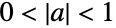

Sqrt[((1 - z) / (1 + z)) ^ 2] - (1 - a) / (1 + a) /. z -> #& /@ %% /. {{a -> (2 + 3I) / 4}, {a -> 2 + 3I}}对于超越方程,SolveValues 可能不会给出所有解:
SolveValues[x + E ^ x == 1 / 2, x]
使用 Reduce 得到所有解:
Reduce[x + E ^ x == 1 / 2, x]SolveValues 通过设置 Method->"Reduce" 使用 Reduce 求解,但返回解的值:
SolveValues[x + E ^ x == 1 / 2, x, Method -> "Reduce"]使用反函数允许 SolveValues 快速得到某些解:
SolveValues[x ^ n == 1, x]//Timing
(red = Reduce[x ^ n == 1, x])//LeafCount//TimingReduce[red /. x -> 2, n]Simplify[x ^ n /. {x -> 2, n -> 2I Pi C[1] / Log[2]}, Element[C[1], Integers]]对假设的解释取决于它们的句法属性. 在此,该解在受假设限制的参数空间中是通用的:
SolveValues[x == a && x == b, x, Assumptions -> a == b]这个数学上等价的假设包含求解变量,因此被当作要求解的系统的一部分:
SolveValues[x == a && x == b, x, Assumptions -> a + x == b + x]SolveValues[x == a && x == b && a + x == b + x, x]SolveValues[x == a && x == b && a + x == b + x, x, MaxExtraConditions -> All]当参数被限定为离散集时,通用性的概念定义不明确,并返回所有解:
SolveValues[a x ^ 2 + b x == 1, x, Assumptions -> Element[a | b, Integers]]SolveValues[(x ^ 2 - 2Sqrt[2]x + 2) / (x - Sqrt[2]) == 0, x]Limit[(x ^ 2 - 2Sqrt[2]x + 2) / (x - Sqrt[2]), x -> Sqrt[2]]SolveValues[x ^ 2 / x == 0, x]
x ^ 2 / x == 0此处, 处的可移除奇点被对方程进行预处理的 Together 取消:
SolveValues[(x ^ 2 - 2x + 1) / (x - 1) == 0, x]Together[(x ^ 2 - 2x + 1) / (x - 1) == 0]MaxRoots 的值仅用于具有数值系数的系统:
SolveValues[x ^ 4 == y, {x, y}, MaxRoots -> 3]SolveValues[x ^ 4 == y, {x}, MaxRoots -> 3]
作为变量给出的表达式被视为原子对象,而不是其子表达式的函数:
SolveValues[x + Sin[x] == 1, Sin[x]]SolveValues[f[x] + Integrate[f[x], {x, 0, 1}] == 2x, f[x]]f[x] + Integrate[f[x], {x, 0, 1}] == 2x /. f[x] -> z文本
Wolfram Research (2021),SolveValues,Wolfram 语言函数,https://reference.wolfram.com/language/ref/SolveValues.html (更新于 2024 年).
CMS
Wolfram 语言. 2021. "SolveValues." Wolfram 语言与系统参考资料中心. Wolfram Research. 最新版本 2024. https://reference.wolfram.com/language/ref/SolveValues.html.
APA
Wolfram 语言. (2021). SolveValues. Wolfram 语言与系统参考资料中心. 追溯自 https://reference.wolfram.com/language/ref/SolveValues.html 年