


StationaryWaveletTransform
StationaryWaveletTransform[data]
gives the stationary wavelet transform (SWT) of an array of data.
StationaryWaveletTransform[data,wave]
gives the stationary wavelet transform using the wavelet wave.
StationaryWaveletTransform[data,wave,r]
gives the stationary wavelet transform using r levels of refinement.
Details and Options
- StationaryWaveletTransform is similar to DiscreteWaveletTransform except that no subsampling occurs at any refinement level and the resulting coefficient arrays all have the same dimensions as the original data.
- StationaryWaveletTransform gives a DiscreteWaveletData object.
- Properties of the DiscreteWaveletData dwd can be found using dwd["prop"], and a list of available properties can be found using dwd["Properties"].
- The data can be any of the following:
-
list arbitrary-rank numerical array image arbitrary Image object audio an Audio or sampled Sound object - The possible wavelets wave include:
-
BattleLemarieWavelet[…] Battle–Lemarié wavelets based on B-spline BiorthogonalSplineWavelet[…] B-spline-based wavelet CoifletWavelet[…] symmetric variant of Daubechies wavelets DaubechiesWavelet[…] the Daubechies wavelets HaarWavelet[…] classic Haar wavelet MeyerWavelet[…] wavelet defined in the frequency domain ReverseBiorthogonalSplineWavelet[…] B-spline-based wavelet (reverse dual and primal) ShannonWavelet[…] sinc function-based wavelet SymletWavelet[…] least asymmetric orthogonal wavelet - The default wave is HaarWavelet[].
- With higher settings for the refinement level r, larger-scale features are resolved.
- The default refinement level r is given by
![TemplateBox[{{{InterpretationBox[{log, _, DocumentationBuild`Utils`Private`Parenth[2]}, Log2, AutoDelete -> True], (, n, )}, +, {1, /, 2}}}, Floor]](Files/StationaryWaveletTransform.en/1.png "TemplateBox[{{{InterpretationBox[{log, _, DocumentationBuild`Utils`Private`Parenth[2]}, Log2, AutoDelete -> True], (, n, )}, +, {1, /, 2}}}, Floor]") , where
, where  is the minimum dimension of data. »
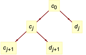
 - The tree of wavelet coefficients at level
 consists of coarse coefficients
  and detail coefficients
  , with
  representing the input data.
 - The forward transform is given by
 and
and  , where
  is the filter length for the corresponding wspec and
  is the length of input data. »
 - The inverse transform is given by
 . »
. » - The
 are lowpass filter coefficients and
  are highpass filter coefficients that are defined for each wavelet family.
 - The dimensions of
 and
and  are the same as input data dimensions.
 - The following options can be given:
-
Method Automatic method to use WorkingPrecision MachinePrecision precision to use in internal computations - StationaryWaveletTransform uses periodic padding of data.
- InverseWaveletTransform gives the inverse transform.
Examples
open all close allBasic Examples (3)
Compute a stationary wavelet transform using the HaarWavelet:
StationaryWaveletTransform[{56, 40, 8, 24, 48, 48, 40, 16}]Use Normal to view all coefficients:
Normal[%]a = Audio["ExampleData/rule30.wav"]dwd = StationaryWaveletTransform[a, Automatic, 3]Use dwd[…,"Audio"] to extract coefficient signals:
dwd[All, "Audio"]Verify lengths of all coefficient signals:
AudioLength[#[[2]]]& /@ %Compute the inverse transform:
InverseWaveletTransform[dwd]Transform an Image object:
dwd = StationaryWaveletTransform[[image], Automatic, 2]Use dwd[…,"Image"] to extract coefficient images:
dwd[All, {"Image", ImageSize -> 80}]Compute the inverse transform:
InverseWaveletTransform[dwd]Scope (34)
Basic Uses (6)
Compute a stationary wavelet transform:
dwd = StationaryWaveletTransform[{0, 0, 1, 0, 0}]The resulting DiscreteWaveletData represents a tree of transform coefficients:
dwd["TreeView"]The inverse transform reconstructs the input:
InverseWaveletTransform[dwd]Useful properties can be extracted from the DiscreteWaveletData object:
dwd = StationaryWaveletTransform[RandomReal[1, {16}], DaubechiesWavelet[4], 2]Get a full list of properties:
dwd["Properties"]Get data and coefficient dimensions:
dwd["DataDimensions"]dwd["Dimensions"]Use Normal to get all wavelet coefficients explicitly:
dwd = StationaryWaveletTransform[Range[4]];Normal[dwd]Also use All as an argument to get all coefficients:
dwd[All]Use Automatic to get only the coefficients used in the inverse transform:
dwd[Automatic]Use the "TreeView" or "IndexMap" to find out what wavelet coefficients are available:
dwd = StationaryWaveletTransform[Range[4], HaarWavelet[], 2];dwd["TreeView"]dwd["IndexMap"]Extract specific coefficient arrays:
dwd[{0}]dwd[{0, 0}]Extract several wavelet coefficients corresponding to the list of wavelet index specifications:
dwd[{{0}, {0, 1}}]Extract all coefficients whose wavelet indexes match a pattern:
dwd[{_}]dwd[{{_, 0}, {_, 1}}]The Automatic coefficients are used by default in functions like WaveletListPlot:
dwd = StationaryWaveletTransform[Table[Sin[x ^ 2], {x, 0, 10, 0.2}], Automatic, 4];First /@ dwd[Automatic]WaveletListPlot[dwd, FrameTicks -> Full]Use a higher refinement level to increase the frequency resolution:
data = Table[Sin[x ^ 2] + RandomReal[{-0.2, 0.2}], {x, 0, 10, 0.02}];ListLinePlot[data]With a smaller refinement level, more of the signal energy is left in {0,0,0}:
dwt1 = StationaryWaveletTransform[data, DaubechiesWavelet[4], 3];WaveletListPlot[dwt1, PlotLayout -> "CommonYAxis"]With further refinement, {0,0,0} is resolved into further components:
dwt2 = StationaryWaveletTransform[data, DaubechiesWavelet[4], 4];WaveletListPlot[dwt2, PlotLayout -> "CommonYAxis"]Wavelet Families (10)
Compute the stationary wavelet transform using different wavelet families:
data = Table[Sin[x ^ 2], {x, 0, 10, 0.02}];dwd1 = StationaryWaveletTransform[data, DaubechiesWavelet[4], 3];
dwd2 = StationaryWaveletTransform[data, SymletWavelet[4], 3];{WaveletListPlot[dwd1, PlotLayout -> "CommonXAxis"], WaveletListPlot[dwd2, PlotLayout -> "CommonXAxis"]}Use different families of wavelets to capture different features:
data = Table[4 Exp[-100 (t - 0.5) ^ 2] + Sin[5Pi t], {t, 0, 1, 0.01}];ListLinePlot[data]HaarWavelet (default):
dwd = StationaryWaveletTransform[data, HaarWavelet[], 3];WaveletListPlot[dwd, PlotLayout -> "CommonYAxis", Filling -> Axis]data = Table[4 Exp[-100 (t - 0.5) ^ 2] + Sin[5Pi t], {t, 0, 1, 0.01}];dwd = StationaryWaveletTransform[data, DaubechiesWavelet[2], 3];WaveletListPlot[dwd, PlotLayout -> "CommonYAxis", Filling -> Axis]data = Table[4 Exp[-100 (t - 0.5) ^ 2] + Sin[5Pi t], {t, 0, 1, 0.01}];dwd = StationaryWaveletTransform[data, BattleLemarieWavelet[3], 3];WaveletListPlot[dwd, PlotLayout -> "CommonYAxis", Filling -> Axis]data = Table[4 Exp[-100 (t - 0.5) ^ 2] + Sin[5Pi t], {t, 0, 1, 0.01}];dwd = StationaryWaveletTransform[data, BiorthogonalSplineWavelet[4, 2], 3];WaveletListPlot[dwd, PlotLayout -> "CommonYAxis", Filling -> Axis]data = Table[4 Exp[-100 (t - 0.5) ^ 2] + Sin[5Pi t], {t, 0, 1, 0.01}];dwd = StationaryWaveletTransform[data, CoifletWavelet[2], 3];WaveletListPlot[dwd, PlotLayout -> "CommonYAxis", Filling -> Axis]data = Table[4 Exp[-100 (t - 0.5) ^ 2] + Sin[5Pi t], {t, 0, 1, 0.01}];dwd = StationaryWaveletTransform[data, MeyerWavelet[3], 3];WaveletListPlot[dwd, PlotLayout -> "CommonYAxis", Filling -> Axis]ReverseBiorthogonalSplineWavelet:
data = Table[4 Exp[-100 (t - 0.5) ^ 2] + Sin[5Pi t], {t, 0, 1, 0.01}];dwd = StationaryWaveletTransform[data, ReverseBiorthogonalSplineWavelet[4, 2], 3];WaveletListPlot[dwd, PlotLayout -> "CommonYAxis", Filling -> Axis]data = Table[4 Exp[-100 (t - 0.5) ^ 2] + Sin[5Pi t], {t, 0, 1, 0.01}];dwd = StationaryWaveletTransform[data, ShannonWavelet[8], 3];WaveletListPlot[dwd, PlotLayout -> "CommonYAxis", Filling -> Axis]data = Table[4 Exp[-100 (t - 0.5) ^ 2] + Sin[5Pi t], {t, 0, 1, 0.01}];dwd = StationaryWaveletTransform[data, SymletWavelet[3], 3];WaveletListPlot[dwd, PlotLayout -> "CommonYAxis", Filling -> Axis]Vector Data (6)
Plot the coefficients over a common horizontal axis using WaveletListPlot:
dwd = StationaryWaveletTransform[Table[Sin[x ^ 2], {x, 0, 10, 0.02}], Automatic, 3];WaveletListPlot[dwd, FrameTicks -> Full]Plot against a common vertical axis:
WaveletListPlot[dwd, PlotLayout -> "CommonYAxis"]Visualize coefficients as a function of time and refinement level using WaveletScalogram:
dwd = StationaryWaveletTransform[Table[Sin[20x] + Sin[10x], {x, 1, 10, 0.01}], Automatic, 4];The coefficient indexes appear as tooltips when the mouse pointer is moved over a coefficient:
WaveletScalogram[dwd, All]data = Table[1, {x, 0, 10, 0.02}];ListLinePlot[data]All coefficients are small except coarse coefficients {0,0,…}:
dwd = StationaryWaveletTransform[data, DaubechiesWavelet[4], 3];WaveletListPlot[dwd, All, PlotLayout -> "CommonYAxis", Filling -> Axis]Data oscillating at the highest resolvable frequency (Nyquist frequency):
data = Table[(-1)^n, {n, 80}];ListLinePlot[data]Only the first detail coefficient {1} is nonzero:
dwd = StationaryWaveletTransform[data, Automatic, 3];WaveletListPlot[dwd, All, PlotLayout -> "CommonYAxis"]Data with large discontinuities:
data = Table[Piecewise[{{1, 1 < x < 3.1}}, 0], {x, 0, 4, 0.02}];ListLinePlot[data]Coarse coefficients {0,…} have the same large-scale structure as the data:
dwd = StationaryWaveletTransform[data, Automatic, 3];WaveletListPlot[dwd, {0..}, FrameTicks -> Full]Detail coefficients are sensitive to discontinuities:
WaveletListPlot[dwd, Except[{0..}], FrameTicks -> Full]Data with both spatial and frequency structure:
data = Table[Piecewise[{{5, n <= 30}, {2 + (-1)^n, Inequality[30, Less, n, LessEqual, 60]}, {5, 60 < n}}], {n, 90}];ListLinePlot[data, PlotRange -> {0, 5}]Coarse coefficients {0,…} track the local mean of the data:
dwd = StationaryWaveletTransform[data, Automatic, 3];WaveletListPlot[dwd, {0..}, FrameTicks -> Full]The first detail coefficient identifies the oscillatory region:
WaveletListPlot[dwd, {1, 0...}, FrameTicks -> Full]All coefficients on a common vertical axis:
WaveletListPlot[dwd, All, PlotLayout -> "CommonYAxis"]Matrix Data (5)
Compute a two-dimensional stationary wavelet transform:
dwd = StationaryWaveletTransform[(| | | | | |
| - | - | - | - | - |
| 0 | 0 | 1 | 0 | 0 |
| 0 | 1 | 1 | 1 | 0 |
| 1 | 1 | 1 | 1 | 1 |
| 0 | 1 | 1 | 1 | 0 |
| 0 | 0 | 1 | 0 | 0 |)]View the tree of wavelet coefficients:
dwd[{"TreeView", Left}]Inverse transform to get back the original signal:
InverseWaveletTransform[dwd]//Chop//MatrixFormUse dwd[…,"MatrixPlot"] to visualize each coefficient as a MatrixPlot:
dwd = StationaryWaveletTransform[DiamondMatrix[32], Automatic, 1]dwd[All, "MatrixPlot"]Visualize wavelet coefficients at higher refinement levels:
dwd2 = StationaryWaveletTransform[DiamondMatrix[32], Automatic, 2];dwd2[All, "MatrixPlot"]In two dimensions, the vector of filtering operations in each direction can be computed:
Tuples[{0, 1}, 2] /. {0 -> "lowpass", 1 -> "highpass"}Interpreting these vectors as binary digit expansions, you get wavelet index numbers:
FromDigits[#, 2]& /@ Tuples[{0, 1}, 2]Get the lowpass and highpass filters for a Haar wavelet:
{lp, hp} = Map[Last, WaveletFilterCoefficients[HaarWavelet[], {"PrimalLowpass", "PrimalHighpass"}], {2}]The resulting 2D filters are outer products of filters in the two directions:
Apply[KroneckerProduct, Tuples[{lp, hp}, 2], {1}]Map[MatrixPlot, %]Wavelet transform of step data:
step[{a_, b_, c_, d_}] :=
	ArrayFlatten[{{ConstantArray[a, {3, 3}], ConstantArray[b, {3, 5}]}, {ConstantArray[c, {5, 3}], ConstantArray[d, {5, 5}]}}];
Data with a vertical discontinuity:
MatrixPlot[step[{0, 1, 0, 1}], FrameTicks -> False]Only the vertical detail coefficients, wavelet index {…,1}, are nonzero:
StationaryWaveletTransform[step[{0, 1, 0, 1}]][Automatic, {"MatrixPlot", ImageSize -> 40}]Data with horizontal discontinuity:
MatrixPlot[step[{0, 0, 1, 1}], FrameTicks -> False]Only the horizontal detail coefficients, wavelet index {…,2}, are nonzero:
StationaryWaveletTransform[step[{0, 0, 1, 1}]][Automatic, {"MatrixPlot", ImageSize -> 40}]Array Data (2)
Compute a three-dimensional stationary wavelet transform:
data = RandomReal[1, {16, 16, 16}];dwd = StationaryWaveletTransform[data, Automatic, 2]Tree view of all coefficients:
dwd["TreeView"]Inverse transform to get back the original signal:
Norm[Flatten[data - InverseWaveletTransform[dwd]]]Wavelet transform of a three-dimensional cross array:
data = CrossMatrix[All, {8, 8, 8}];Graphics3D[{Red, Cuboid /@ Position[data, 1]}]dwd = StationaryWaveletTransform[data, Automatic, 1]Visualize wavelet coefficients:
Table[i -> Graphics3D[{If[Positive[Extract[dwd[i][[1, 2]], #]], Red, Green], Cuboid[#]}& /@ Position[dwd[i][[1, 2]], u_ /; Abs[u] > 0], PlotRange -> {{1, 9}, {1, 9}, {1, 9}}], {i, dwd["IndexMap"]}]Energy of the original data is conserved within the transformed coefficients:
Total[Flatten[data]^2] == Total[Flatten[dwd[Automatic][[All, 2]]]^2]Image Data (2)
Transform an Image object:
img = Image[DiamondMatrix[All, {64, 64}]]dwd = StationaryWaveletTransform[img, HaarWavelet[], 3]The inverse transform yields a reconstructed Image object:
InverseWaveletTransform[dwd]Wavelet coefficients are normally given as arrays of data for each image channel:
dwd = StationaryWaveletTransform[[image], HaarWavelet[], 2];Dimensions[{0, 0} /. Normal[dwd]]Number of channels and dimensions of the original image are the same:
Dimensions[ImageData[[image], Interleaving -> False]]Get all coefficients as Image objects instead of arrays of data:
dwd[All, "Image"]Get raw Image objects with no rescaling of color levels:
dwd[All, {"Image", "ImageFunction" -> Identity}]Get the inverse transform of the {0,1} coefficient as an Image object:
dwd[{0, 1}, {"Image", "Inverse"}]Sound Data (3)
Transform a Sound object:
snd = ExampleData[{"Sound", "Apollo11ReturnSafely"}]dwd = StationaryWaveletTransform[snd]The inverse transform yields a reconstructed Sound object:
InverseWaveletTransform[dwd]By default, coefficients are given as lists of data for each sound channel:
dwd = StationaryWaveletTransform[ExampleData[{"Sound", "PianoScale"}]];Dimensions[{0, 0, 1} /. Normal[dwd]]Number of channels and data length in the original sound are the same:
Dimensions[First[First[ExampleData[{"Sound", "PianoScale"}]]]]Get the {0,1} coefficient as a Sound object:
dwd[{0, 0, 1}, "Sound"]Inverse transform of {0,0,1} coefficient as a Sound object:
dwd[{0, 0, 1}, {"Sound", "Inverse"}]Browse all coefficients using a MenuView:
dwd = StationaryWaveletTransform[ExampleData[{"Sound", "Clarinet"}], SymletWavelet[3], 3];MenuView[dwd[All, "Sound"]]Generalizations & Extensions (3)
StationaryWaveletTransform works on arrays of symbolic quantities:
dwd = StationaryWaveletTransform[{a, b, c, d}, WorkingPrecision -> ∞];Normal[dwd]//SimplifyInverse transform recovers the input exactly:
InverseWaveletTransform[dwd]//SimplifySpecify any internal working precision:
dwd = StationaryWaveletTransform[{1, 2, 5, 3}, WorkingPrecision -> 20];dwd[Automatic]data = Exp[I RandomReal[1, 4]];dwd = StationaryWaveletTransform[data]The wavelets coefficients are complex:
dwd[Automatic]Inverse transform recovers the input:
Norm[InverseWaveletTransform[dwd] - data]Options (3)
WorkingPrecision (3)
By default, WorkingPrecision->MachinePrecision is used:
data = RandomInteger[1, {10}];dwd1 = StationaryWaveletTransform[data]dwd2 = StationaryWaveletTransform[data, WorkingPrecision -> MachinePrecision]dwd1 == dwd2Use higher-precision computation:
data = {0, 0, 1, 1};dwd = Normal@StationaryWaveletTransform[data, WorkingPrecision -> 25]{Precision[dwd], Accuracy[dwd]}Use WorkingPrecision->∞ for exact computation:
data = RandomInteger[10, {4}];Normal@StationaryWaveletTransform[data, WorkingPrecision -> ∞]//SimplifyApplications (3)
Inverse Halftoning (1)
A simple wavelet-based inverse halftoning:
img = ImageTake[ [image], 100]swt = StationaryWaveletTransform[img, DaubechiesWavelet[4], 2];Apply GaussianFilter on the detail coefficients:
InverseWaveletTransform[WaveletMapIndexed[GaussianFilter[#, 4]&, swt, Except[{___, 0}]]]Numerical Differentiation (1)
Differentiate noisy data using wavelet transform:
f[x_] := Log[2 + Sin[3 π Sqrt[x]]]{t, fd} = Transpose[Table[{x, f[x] + RandomReal[NormalDistribution[0, 0.01]]}, {x, 0.01, 1, 0.001}]];ListLinePlot[fd]Translation-Rotation-Transform (TRT) is used to reduce boundary effects by subtracting a linear component from the input signal:
a = (Max[fd] - Min[fd]/Max[t] - Min[t]);b = Min[fd] - a Min[t];Subscript[fd, TRT] = fd - (a t + b);Since HaarWavelet has one vanishing moment, choose it to perform a wavelet transform on ![]() :
:
wd = StationaryWaveletTransform[Subscript[fd, TRT], HaarWavelet[], 4];j = wd["Refinement"];Detail coefficients give the differentiation of the data. Coefficients at refinement level 4 are chosen to minimize noise:
du = Sqrt[2]^jFirst[wd[{0, 0, 0, 1}, "Values"]];Rescale the differentiated values:
dx = 0.001;dudx = (4 du /dx (2^j)^(3/2)) + a;Compare wavelet-based numerical differentiation with exact differentiation:
Show[ListLinePlot[Transpose[{t, dudx}]], Plot[Evaluate[D[f[x], x]], {x, 0.01, 1}, PlotStyle -> Red], PlotRange -> All]Compare with standard Wolfram Language numerical differentiation:
ifunc = Interpolation[Transpose[{t, fd}]];Plot[ifunc'[x], {x, 0.01, 1}]Image Fusion (1)
Add texture to an existing image:
{img, txt} = { [image], [image]};Perform wavelet transform on both images:
dwd1 = StationaryWaveletTransform[img, CDFWavelet[], 3];dwd2 = StationaryWaveletTransform[txt, CDFWavelet[], 3];Combine detail coefficients of the two images by taking their mean:
rval1 = dwd1[{___, 1 | 2 | 3}, "Values"];rval2 = dwd2[{___, 1 | 2 | 3}, "Values"];wind = Cases[dwd1["WaveletIndex"], {___, 1 | 2 | 3}];nimg = (Image[#1, Interleaving -> False]&) /@ ((1/2) (rval1 + 2 rval2));rnew = MapThread[Rule, {wind, nimg}];Append the coarse coefficient of the first image:
rr = Append[rnew, First[dwd1[{0, 0, 0}, {"Image", "ImageFunction" -> Identity}]]];Construct a new DiscreteWaveletData of the combined wavelet coefficients:
dwdnew = DiscreteWaveletData[rr, CDFWavelet[], StationaryWaveletTransform]Reconstruct the combined image:
InverseWaveletTransform[dwdnew]Properties & Relations (12)
StationaryWaveletPacketTransform computes the full tree of wavelet coefficients:
swpt = StationaryWaveletPacketTransform[{1, 1, 3, 1, 1}];swpt[{"TreeView", Left}]StationaryWaveletTransform computes a subset of the full tree of coefficients:
swt = StationaryWaveletTransform[{1, 1, 3, 1, 1}];swt[{"TreeView", Left}]DiscreteWaveletTransform coefficients halve in length with each level of refinement:
Normal[DiscreteWaveletTransform[{1, 2, 3, 4}]]Rotated data gives different coefficients:
Normal[DiscreteWaveletTransform[{2, 3, 4, 1}]]StationaryWaveletTransform coefficients have the same length as the original data:
Normal[StationaryWaveletTransform[{1, 2, 3, 4}]]Rotated data gives rotated coefficients:
Normal[StationaryWaveletTransform[{2, 3, 4, 1}]]The default refinement is given by ![]() :
:
data = RandomReal[1, {100}];r = Floor[Log2[Length[data]] + (1/2)]StationaryWaveletTransform[data] == StationaryWaveletTransform[data, Automatic, r]data = RandomReal[1, {100, 10, 10}];r = Floor[Log2[Min[Dimensions[data]]] + (1/2)]StationaryWaveletTransform[data] == StationaryWaveletTransform[data, Automatic, r]The energy norm is conserved for orthogonal wavelet families:
data = RandomReal[1, {100}];swt = StationaryWaveletTransform[data];Norm[data] == Norm[Flatten[Last /@ swt[Automatic]]]The energy norm is approximately conserved for biorthogonal wavelet families:
data = RandomReal[1, {100}];swt = StationaryWaveletTransform[data, BiorthogonalSplineWavelet[2, 4]];Norm[data]Norm[Flatten[Last /@ swt[Automatic]]]The mean of the data is captured at the maximum refinement level of the transform:
data = RandomReal[1, 16];swt = StationaryWaveletTransform[data, HaarWavelet[]];Extract the coefficient for the maximum refinement level:
r = swt["Refinement"]swt[ConstantArray[0, {r}]]Mean[data]The sum of inverse transforms from individual coefficient arrays gives the original data:
data = Table[DiscreteDelta[n], {n, -2, 2}]dwt = StationaryWaveletTransform[data];dwt["TreeView"]Individually inverse transform each wavelet coefficient array:
data1 = InverseWaveletTransform[dwt, Automatic, {0, 0}]data2 = InverseWaveletTransform[dwt, Automatic, {0, 1}]data3 = InverseWaveletTransform[dwt, Automatic, {1}]The sum gives the original data:
data1 + data2 + data3Compute stationary wavelet coefficients for periodic data:
x = Range[8];dwd = StationaryWaveletTransform[x, HaarWavelet[]];J = dwd["Refinement"];
l = First[ dwd["DataDimensions"]];a = WaveletFilterCoefficients[HaarWavelet[], "PrimalLowpass"][[All, 2]];
b = WaveletFilterCoefficients[HaarWavelet[], "PrimalHighpass"][[All, 2]];f = Length[a];Coarse coefficients at level ![]() are given by
are given by ![]() :
:
SetAttributes[c, Listable];c[0, n_] := x[[n]];
c[j_, n_] := Underoverscript[∑, m = 1, f]a[[m]] c[j - 1, Mod[n + 2^j - 1(1 - Mod[m, l]), l, 1]]dwd[{___, 0}, "Values"] == Table[c[j, Range[l]], {j, 1, J}]Detail coefficients at level ![]() are given by
are given by ![]() :
:
SetAttributes[d, Listable];d[j_, n_] := Underoverscript[∑, m = 1, f]b[[m]] c[j - 1, Mod[n + 2^j - 1 (1 - Mod[m, l]), l, 1]]dwd[{___, 1}, "Values"] == Table[d[j, Range[l]], {j, 1, J}]Compute partial stationary inverse wavelet transform:
x = Range[8];dwd = StationaryWaveletTransform[x, HaarWavelet[]];J = dwd["Refinement"];
l = First[ dwd["DataDimensions"]];a = WaveletFilterCoefficients[HaarWavelet[], "PrimalLowpass"][[All, 2]];
b = WaveletFilterCoefficients[HaarWavelet[], "PrimalHighpass"][[All, 2]];f = Length[a];Coarse coefficients at level ![]() are given:
are given:
SetAttributes[c, Listable];c[0, n_] := x[[n]];
c[j_, n_] := c[j, n] = Underoverscript[∑, m = 1, f]a[[m]] c[j - 1, Mod[n + 2^j - 1(1 - Mod[m, l]), l, 1]]Detail coefficients at level ![]() are given:
are given:
SetAttributes[d, Listable];d[j_, n_] := d[j, n] = Underoverscript[∑, m = 1, f]b[[m]] c[j - 1, Mod[n + 2^j - 1 (1 - Mod[m, l]), l, 1]]Inverse wavelet transform at level ![]() is given by
is given by ![]() :
:
SetAttributes[iwt, Listable];iwt[j_Integer, n_Integer] := Underoverscript[∑, m = 1, f](a[[m]] c[j + 1, Mod[n + 2^j(-1 + Mod[m, l]), l, 1]] + b[[m]] d[j + 1, Mod[n + 2^j (-1 + Mod[m, l]), l, 1]])Reconstruct coarse coefficients {0,0} at refinement level ![]() :
:
iwt[2, Range[l]] == First[dwd[{0, 0}, "Values"]]Reconstruct coarse coefficients {0} at refinement level ![]() :
:
iwt[1, Range[l]] == First[dwd[{0}, "Values"]]Compute a Haar stationary wavelet transform in one dimension:
low[v_] := ListCorrelate[{1 / 2, 1 / 2}, v, -1]
high[v_] := ListCorrelate[{-1 / 2, 1 / 2}, v, -1]HaarSWT[v_] := {{0} -> low[v], {1} -> high[v]};Compute {0} and {1} wavelet coefficients:
HaarSWT[{a, b, c, d}]Compare with DiscreteWaveletPacketTransform:
StationaryWaveletTransform[{a, b, c, d}, HaarWavelet[], 1, WorkingPrecision -> ∞][All]In two dimensions, a separate filter is applied in each dimension:
f2d[fx_, fy_] := Composition[Map[fy, #]&, Map[fx, #]&]Lowpass and highpass filters for a Haar wavelet:
low[v_] := ListCorrelate[{1 / 2, 1 / 2}, v, -1]
high[v_] := ListCorrelate[{-1 / 2, 1 / 2}, v, -1]
Haar wavelet transform of matrix data:
data = Table[Sin[x y], {x, -2, 2, 4 / 63}, {y, -2, 2, 4 / 63}];Table[MatrixPlot[f2d[fx, fy][data], PlotLabel -> {fx, fy}, FrameTicks -> None], {fx, {low, high}}, {fy, {low, high}}]//FlattenCompare with DiscreteWaveletPacketTransform using HaarWavelet:
dwd = StationaryWaveletTransform[data, HaarWavelet[], 1];Table[MatrixPlot[Last[p], PlotLabel -> First[p], FrameTicks -> None], {p, Normal[dwd]}]Image channels are transformed individually:
dwds = Map[StationaryWaveletTransform, ColorSeparate[[image]]];Combine {0} coefficients of separately transformed image channels:
w = Image[Table[Part[t[{0}, "Values"], 1, 1], {t, dwds}], Interleaving -> False]Compare with {0} coefficient of StationaryWaveletTransform of the original image:
dwd = StationaryWaveletTransform[[image]];First[dwd[{0}, {"Values", {"Image", "ImageFunction" -> Identity}}]]ImageSubtract[w, %]Text
Wolfram Research (2010), StationaryWaveletTransform, Wolfram Language function, https://reference.wolfram.com/language/ref/StationaryWaveletTransform.html (updated 2017).
CMS
Wolfram Language. 2010. "StationaryWaveletTransform." Wolfram Language & System Documentation Center. Wolfram Research. Last Modified 2017. https://reference.wolfram.com/language/ref/StationaryWaveletTransform.html.
APA
Wolfram Language. (2010). StationaryWaveletTransform. Wolfram Language & System Documentation Center. Retrieved from https://reference.wolfram.com/language/ref/StationaryWaveletTransform.html