


ComplexRegionPlot
ComplexRegionPlot[pred,{z,zmin,zmax}]
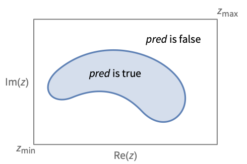
pred がTrueとなる複素平面上の領域を示すプロットを作成する.
ComplexRegionPlot[{pred1,pred2,…},{z,zmin,zmax}]
複数の述語 prediによって与えられた領域をプロットする.
詳細とオプション
- 述語 prediは不等式の任意の論理結合でよい.prediは,比較の目的で複素数から実数成分を抽出する,Re,Im,Abs,Argのような関数を含むことが多い.
- ComplexRegionPlotがプロットする領域には不連続の部分が含まれていてもよい.
- ComplexRegionPlot[pred,{z,n}]はComplexRegionPlot[pred,{z,-n-n I,n+n I}]と等価である.
- ComplexRegionPlotは,事実上Blockを使って,変数 z を局所的なものとして扱う.
- ComplexRegionPlotには属性HoldAllがあり,z に特定の数値を割り当てた後ではじめて pred を評価する.場合によっては,Evaluateを使ってまず pred を記号的に評価した方が効率的かもしれない.
- prediには次のラッパー w を使うことができる.
-
Annotation[predi,label] prediの注釈を与える Button[predi,action] prediの曲線がクリックされたときに action を評価する Callout[predi,label] コールアウトで領域にラベルを付ける Callout[predi,label,pos] コールアウトを相対的な位置 pos に置く EventHandler[predi,events] prediの一般的なイベントハンドラを定義する Hyperlink[predi,uri] 領域をハイパーリンクにする Labeled[predi,label] 領域にラベルを付ける Labeled[predi,label,pos] ラベルを相対的な位置 pos に置く Legended[predi,label] 領域を凡例で識別する PopupWindow[predi,cont] 領域にポップアップウィンドウを付ける StatusArea[predi,label] マウスオーバーの際にステータスエリアに表示する Style[predi,styles] 領域を指定のスタイルで表示する Tooltip[predi,label] 領域にツールチップを付ける Tooltip[predi] 領域をツールチップとして使う - ラッパー w は複数のレベルで適用できる.
-
w[predi] prediをラップする w[{predi,…}] prediの集合をラップする w1[w2[…]] ネストしたラッパーを使う - Callout,Labeled,Placedには次の位置 pos が使える.
-
Automatic 自動的に置かれたラベル Above, Below, Before, After 曲線の周囲の位置 z z 近くの位置 {pos,epos} 領域の相対的な位置 pos に置かれたラベル内の epos - ComplexRegionPlotにはGraphicsと同じオプションに以下の追加・変更を加えたものが設定できる. [全オプションのリスト]
-
AspectRatio 1 縦横比 BoundaryStyle Automatic 各領域の境界のスタイル ColorFunction Automatic 各領域の内側の彩色をどうするか ColorFunctionScaling True ColorFunctionの引数をスケールするかどうか EvaluationMonitor None 各関数評価で評価される式 Frame True プロットの周囲に枠を描くかどうか LabelingSize Automatic コールアウトとラベルの最大サイズ MaxRecursion Automatic 許容される再帰分割の最大数 Mesh None メッシュラインを何本引くか MeshFunctions {#1&,#2&} どのようなメッシュラインを描くか MeshShading None メッシュライン間の領域の陰影付けをどうするか MeshStyle Automatic メッシュラインのスタイル Method Automatic 領域を細分化するためのメソッド PerformanceGoal $PerformanceGoal パフォーマンスのどの面について最適化するか PlotLabels None 曲線に使うラベル PlotLegends None 領域の凡例 PlotPoints Automatic サンプル点の初期数 PlotRange Full プロットに含める値の範囲 PlotRangeClipping True プロット範囲で切り取るかどうか PlotRangePadding Automatic 値の範囲をどの程度充填するか PlotStyle Automatic 領域のスタイルを指定するグラフィックス指示子 PlotTheme $PlotTheme プロットの全体的なテーマ TextureCoordinateFunction Automatic テクスチャ座標をどのように決めるか TextureCoordinateScaling True TextureCoordinateFunctionの引数をスケールするかどうか WorkingPrecision MachinePrecision 内部計算に使われる精度 - 次は,PlotLegendsのよく使われる設定である.
-
None 凡例は付けない Automatic 凡例を自動的に決定する "Expressions" f1, f2, … を凡例ラベルとして使う {lbl1,lbl2,…} lbl1, lbl2, … を凡例ラベルとして使う Placed[lspec,…] 凡例の置き方を指定する - PlotStylesty は,各曲線に使用するスタイルを指定する.取り得る設定には以下がある.
-
{sty1,sty2,…} データ集合に対するスタイルの列 <"key"val,…> データの異なるレベルに対するスタイル要素 - 使用可能なキーは次の通りである.
-
"Base" すべての fiに対する全体的なスタイル "Functions" 各 fi に対するスタイル styiのリスト - ColorData["DefaultPlotColors"]は,PlotStyleによって使用されるデフォルトの色の並びを与える.
- ComplexRegionPlotは,まず,PlotPointsで指定された等間隔のサンプル点の格子で pred を評価する.次に,pred がTrueとなるすべての領域の境界を見付けるために,適応的アルゴリズムを使って最大でMaxRecursion回再分割する.
- 使うサンプル点の数が有限なので,pred がTrueとなる領域をComplexRegionPlotが見逃す可能性がある点に留意する必要がある.結果をチェックする際は,PlotPointsおよびMaxRecursionの設定を大きくするとよい.
- デフォルト設定のPlotRange->Fullのとき,ComplexRegionPlotは z の全範囲(zminから zmaxまで)を明示的に含む.
- ComplexRegionPlotは,一般に,正の領域のみを求める.線あるいは点のみの領域は求められない.
- MeshFunctions内の関数に渡される引数は z である.ColorFunctionとTextureCoordinateFunctionには,デフォルトで,Re[z],Im[z],Abs[z],Arg[z]のスケールされたバージョンが渡される.
全オプションのリスト
例題
すべて開く すべて閉じる例 (5)
ComplexRegionPlot[Abs[z] ≤ 1, {z, -1 - I, 1 + I}]{z,1}で領域を指定することは{z,-1-,1+}と同じである:
ComplexRegionPlot[Abs[z] ≤ 1, {z, 1}]ComplexRegionPlot[0 < Arg[z] < 2π / 3, {z, 5}]ComplexRegionPlot[{Re[z ^ 2] < 1, Im[z ^ 2] < 1}, {z, 2}]ComplexRegionPlot[Abs[z] ≤ 1 && Abs[Arg[z]] > π / 4, {z, -1 - I, 1 + I}, PlotStyle -> Yellow]スコープ (23)
サンプリング (3)
ComplexRegionPlot[Abs[Nest[(# ^ 2 + z)&, z, 8]] < 2, {z, -2 - 1.5I, 1 + 1.5I}, Mesh -> All]PlotPointsとMaxRecursionを使って適応的サンプリングを制御する:
Table[ComplexRegionPlot[1 < Abs[Sin[2 z] Cosh[2 z]] < 4, {z, -2 - 2I, 2 + 2I}, PlotPoints -> pp, MaxRecursion -> mr, Mesh -> None], {mr, {0, 2}}, {pp, {5, 15}}]ComplexRegionPlot[Re[z^2] ≤ 2 && Im[z^2] > 1, {z, -3 - 3I, 3 + 3I}]ラベルと凡例 (9)
Labeledで領域にラベルを付ける:
ComplexRegionPlot[Labeled[Abs[z] < 1, "disk", Above], {z, -1.5 - 1.5I, 1.5 + 1.5I}]ComplexRegionPlot[{Labeled[Abs[z] < 1, "disk", Right], Labeled[Re[z] < 1, "rectangle", Below]}, {z, -1.5 - 1.5I, 1.5 + 1.5I}]Table[ComplexRegionPlot[Labeled[Abs[z] < 1, "disk", pos], {z, -1.5 - 1.5I, 1.5 + 1.5I}, PlotLabel -> pos], {pos, {Top, Bottom, Left, Right}}]Calloutで領域にラベルを付ける:
ComplexRegionPlot[Callout[1 < Abs[Sin[2 z] Sinh[2 z]] < 6, "region", {1, 1}], {z, -2 - 2I, 2 + 2I}]ComplexRegionPlot[{Callout[1 < Abs[Sin[2 z] Sinh[2 z]] < 6, "region", {1, 1}], Callout[Abs[z] < 2, "disk", {1, -1}]}, {z, -2 - 2I, 2 + 2I}]ラベルが領域内にあるときはコールアウトのリーダー線は使われない:
ComplexRegionPlot[Callout[Abs[Sin[2 z] Sinh[2 z]] < 6, "region", {0, 0}], {z, -2 - 2I, 2 + 2I}]PlotLegendsで凡例を加える:
ComplexRegionPlot[{1 < Abs[Sin[2 z] Sinh[2 z]] < 6, Abs[z] < 2}, {z, -2 - 2I, 2 + 2I}, PlotLegends -> "Expressions"]ComplexRegionPlot[{1 < Abs[Sin[2 z] Sinh[2 z]] < 6, Abs[z] < 2}, {z, -2 - 2I, 2 + 2I}, PlotLegends -> Automatic]Legendedで凡例を加える:
ComplexRegionPlot[{Legended[1 < Abs[Sin[2 z] Sinh[2 z]] < 6, "region"], Legended[Abs[z] < 2, "disk"]}, {z, -2 - 2I, 2 + 2I}]プレゼンテーション (11)
領域に明示的なPlotStyleを与える:
ComplexRegionPlot[Abs[z] ≤ 1 && Abs[Arg[z]] > π / 4, {z, -1 - I, 1 + I}, PlotStyle -> Yellow]領域の境界に明示的なBoundaryStyleを与える:
ComplexRegionPlot[Abs[z] ≤ 1 && Abs[Arg[z]] > π / 4, {z, -1 - I, 1 + I}, PlotStyle -> Yellow, BoundaryStyle -> Dashed]ComplexRegionPlot[{3 ≤ Abs[z] ≤ 4, Abs[z] < 2}, {z, -4 - 4I, 4 + 4I}, FrameLabel -> {"real", "imaginary"}, PlotLabel -> "shapes", PlotLabels -> {"annulus", "disk"}]ComplexRegionPlot[{Callout[3 ≤ Abs[z] ≤ 4, "annulus"], Labeled[Abs[z] < 2, "disk", Below]}, {z, -4 - 4I, 4 + 4I}]ComplexRegionPlot[{3 ≤ Abs[z] ≤ 4, Abs[z] < 2}, {z, -4 - 4I, 4 + 4I}, PlotLegends -> "Expressions"]ComplexRegionPlot[{3 ≤ Abs[z] ≤ 4, Abs[z] < 2}, {z, -4 - 4I, 4 + 4I}, PlotLegends -> Automatic]ComplexRegionPlot[2 ≤ Abs[z] ≤ 4, {z, -4 - 4I, 4 + 4I}, ColorFunction -> Hue, PlotLegends -> Automatic]ComplexRegionPlot[2 ≤ Abs[z] ≤ 4, {z, -4 - 4I, 4 + 4I}, Mesh -> 8, MeshStyle -> Directive[Red, Dashed]]ComplexRegionPlot[2 ≤ Abs[z] ≤ 4, {z, -4 - 4I, 4 + 4I}, Mesh -> 8, MeshShading -> {{Yellow, Orange}, {Pink, Red}}]ComplexRegionPlot[Abs[Nest[(# ^ 2 + z)&, z, 8]] < 2, {z, -2 - 1.5I, 1 + 1.5I}, ColorFunction -> Function[{re, im, abs, arg}, Hue[Nest[(# ^ 2 + re)&, re, 8]]], ColorFunctionScaling -> False, PlotPoints -> 50]ComplexRegionPlot[2 ≤ Abs[z] ≤ 4, {z, -4 - 4I, 4 + 4I}, PlotTheme -> "Scientific"]オプション (59)
BoundaryStyle (4)
ComplexRegionPlot[Abs[z^4 - z / 5 + 1] ≤ 1, {z, -1 - I, 1 + I}]Noneを使うと境界線は表示されない:
ComplexRegionPlot[Abs[z^4 - z / 5 + 1] ≤ 1, {z, -1 - I, 1 + I}, BoundaryStyle -> None]ComplexRegionPlot[Abs[z^4 - z / 5 + 1] ≤ 1, {z, -1 - I, 1 + I}, BoundaryStyle -> Red]ComplexRegionPlot[Abs[z^4 - z / 5 + 1] ≤ 1, {z, -1 - I, 1 + I}, BoundaryStyle -> Directive[Thickness[Medium], Dashed]]ColorFunction (5)
スケールされた,Re[z],Im[z],Abs[z]あるいはArg[z]で領域に彩色する:
{
	ComplexRegionPlot[Abs[z] < 2, {z, -2 - 2I, 2 + 2I}, ColorFunction -> (Hue[#1]&)],
	ComplexRegionPlot[Abs[z] < 2, {z, -2 - 2I, 2 + 2I}, ColorFunction -> (Hue[#2]&)],
	ComplexRegionPlot[Abs[z] < 2, {z, -2 - 2I, 2 + 2I}, ColorFunction -> (Hue[#3]&)],
	ComplexRegionPlot[Abs[z] < 2, {z, -2 - 2I, 2 + 2I}, ColorFunction -> (Hue[#4]&)]
}名前付きの色関数はスケールされたArg[z]方向を使う:
ComplexRegionPlot[Abs[z] < 1, {z, -1 - I, 1 + I}, ColorFunction -> "Rainbow"]
ComplexRegionPlot[Abs[z^4 - z / 5 + 1] ≤ 1, {z, -1 - I, 1 + I}, ColorFunction -> Function[{z}, ColorData["SolarColors"][Abs[z]]], ColorFunctionScaling -> False]ColorFunctionはPlotStyleより優先順位が高い:
ComplexRegionPlot[Abs[z^4 - z / 5 + 1] ≤ 1, {z, -1 - I, 1 + I}, ColorFunction -> "DarkRainbow", PlotStyle -> Directive[Opacity[0.5], Red]]ColorFunctionはMeshShadingより優先順位が低い:
ComplexRegionPlot[Abs[z^4 - z / 5 + 1] ≤ 1, {z, -1 - I, 1 + I}, Mesh -> 30, MeshShading -> {{Gray, Automatic}, {Automatic, Gray}}, ColorFunction -> "DarkRainbow"]ColorFunctionScaling (1)
スケールされていないRe[z],Im[z],Abs[z]あるいはArg[z]を領域の彩色に使う:
{
	ComplexRegionPlot[Abs[z] < 2, {z, -2 - 2I, 2 + 2I}, ColorFunction -> (Hue[#1]&), ColorFunctionScaling -> False],
	ComplexRegionPlot[Abs[z] < 2, {z, -2 - 2I, 2 + 2I}, ColorFunction -> (Hue[#2]&), ColorFunctionScaling -> False],
	ComplexRegionPlot[Abs[z] < 2, {z, -2 - 2I, 2 + 2I}, ColorFunction -> (Hue[#3]&), ColorFunctionScaling -> False],
	ComplexRegionPlot[Abs[z] < 2, {z, -2 - 2I, 2 + 2I}, ColorFunction -> (Hue[#4]&), ColorFunctionScaling -> False]
	}
LabelingSize (2)
ComplexRegionPlot[Callout[Abs[z] ≤ 1 && Abs[Arg[z]] > π / 4, "region"], {z, -1 - I, 1 + I}, PlotStyle -> Yellow]ComplexRegionPlot[Callout[Abs[z] ≤ 1 && Abs[Arg[z]] > π / 4, "region"], {z, -1 - I, 1 + I}, PlotStyle -> Yellow, LabelingSize -> 25]MaxRecursion (1)
Mesh (7)
ComplexRegionPlot[Abs[z] ≤ 1, {z, -1 - I, 1 + I}]{ComplexRegionPlot[Abs[z] ≤ 1, {z, -1 - I, 1 + I}, Mesh -> Full],
ComplexRegionPlot[Abs[z] ≤ 1, {z, -1 - I, 1 + I}, Mesh -> All]}ComplexRegionPlot[Abs[z] ≤ 1, {z, -1 - I, 1 + I}, Mesh -> 10]Re[z]方向に3本のメッシュラインを,Im[z]方向には6本のメッシュラインを使う:
ComplexRegionPlot[Abs[z] ≤ 1, {z, -1 - I, 1 + I}, Mesh -> {3, 6}]ComplexRegionPlot[Abs[z] ≤ 1, {z, -1 - I, 1 + I}, Mesh -> {{-1 / 2, 1 / 2}, {0}}]ComplexRegionPlot[Abs[z] ≤ 1, {z, -1 - I, 1 + I}, Mesh -> {{{-1 / 2, Red}, {1 / 2, Red}}, {{0, Dashed}}}]ComplexRegionPlot[Abs[z] > 1 && Pi / 4 < Abs[Arg[z]] < 3Pi / 4, {z, -2 - 2I, 2 + 2I}, Mesh -> 10]MeshFunctions (2)
{ComplexRegionPlot[Abs[z] ≤ 1, {z, -1 - I, 1 + I}, Mesh -> 10, MeshFunctions -> {Re[#]&}], ComplexRegionPlot[Abs[z] ≤ 1, {z, -1 - I, 1 + I}, Mesh -> 10, MeshFunctions -> {Im[#]&}]}ComplexRegionPlot[Abs[z] ≤ 1, {z, -1 - I, 1 + I}, Mesh -> 10, MeshFunctions -> {Abs[#]&}]MeshShading (4)
Noneを使って領域を取り除く:
ComplexRegionPlot[Abs[z] ≤ 1, {z, -1 - I, 1 + I}, Mesh -> 8, MeshFunctions -> {Re[#] - Im[#]&}, MeshShading -> {Red, None}]ComplexRegionPlot[Abs[z] ≤ 1, {z, -1 - I, 1 + I}, Mesh -> 10, MeshShading -> {{Red, Yellow}, {Pink, Orange}}]MeshShadingはPlotStyleより優先順位が高い:
ComplexRegionPlot[Abs[z] ≤ 1, {z, -1 - I, 1 + I}, Mesh -> 10, PlotStyle -> Blue, MeshShading -> {{Automatic, Green}, {Green, Automatic}}]MeshShadingはColorFunctionより優先順位が高い:
ComplexRegionPlot[Abs[z] ≤ 1, {z, -1 - I, 1 + I}, Mesh -> 10, PlotStyle -> Blue, MeshShading -> {{Automatic, None}, {None, Automatic}}, ColorFunction -> "DarkRainbow"]MeshStyle (2)
PerformanceGoal (2)
PlotLabels (5)
ComplexRegionPlot[1 < Abs[Sin[5 z] Cosh[2z]] < 3, {z, -1 - I, 1 + I}, PlotLabels -> "label"]ComplexRegionPlot[1 < Abs[Sin[5 z] Cosh[2z]] < 3, {z, -1 - I, 1 + I}, PlotLabels -> Placed["island", Above]]ComplexRegionPlot[1 < Abs[Sin[5 z] Cosh[2z]] < 3, {z, -1 - I, 1 + I}, PlotLabels -> Placed["hole", Center]]Calloutを使ってラベルを置く:
ComplexRegionPlot[{1 < Abs[Sin[5 z] Cosh[2z]] < 3}, {z, -1 - I, 1 + I}, PlotLabels -> Callout["label", {0.5, 0.5}]]ComplexRegionPlot[{1 < Abs[Sin[5 z] Cosh[2z]] < 3, Abs[z ^ 2 + 1] > 1}, {z, -1 - I, 1 + I}, PlotLabels -> {Callout["label1", Below], Callout["label2", After]}]PlotLegends (8)
ComplexRegionPlot[Abs[Nest[(# ^ 2 + z)&, z, 8]] < 2, {z, -2 - 1.5I, 1 + 1.5I}, PlotLegends -> All]ComplexRegionPlot[{1 < Abs[Sin[5 z] Cosh[2z]] < 3, Abs[z ^ 2 + 1] > 1}, {z, -1 - I, 1 + I}, PlotLegends -> Automatic]ComplexRegionPlot[Abs[z] ≤ 1, {z, -1 - I, 1 + I}, ColorFunction -> "GreenPinkTones", PlotLegends -> Automatic]PlotLegendsはスタイルを自動的に選ぶ:
ComplexRegionPlot[{Abs[z ^ 2 + 1] > 1, 1 < Abs[Sin[5 z] Cosh[2z]] < 3}, {z, -1 - I, 1 + I}, PlotStyle -> {StandardRed, StandardBlue}, PlotLegends -> Automatic]ComplexRegionPlot[{1 < Abs[Sin[5 z] Cosh[2z]] < 3, Abs[z ^ 2 + 1] > 1}, {z, -1 - I, 1 + I}, PlotLegends -> "Expressions"]ComplexRegionPlot[{Abs[z - 1] < 1, Abs[z + 1] < 1}, {z, -2 - 2I, 2 + 2I}, PlotLegends -> {"left", "right"}]Placedを使って凡例の位置を変える:
Table[ComplexRegionPlot[{Abs[z - 1] < 1, Abs[z + 1] < 1}, {z, -2 - 2I, 2 + 2I}, PlotLegends -> Placed[Automatic, pos], PlotLabel -> pos], {pos, {Before, After, Above, Below}}]SwatchLegendを使って凡例の外観を変える:
ComplexRegionPlot[{Abs[z - 1] < 1, Abs[z + 1] < 1}, {z, -2 - 2I, 2 + 2I}, PlotLegends -> SwatchLegend[Automatic, {"right", "left"}, LegendFunction -> "Frame", LegendLabel -> "ℛ"]]PlotPoints (1)
PlotRange (2)
PlotStyle (5)
ComplexRegionPlot[Abs[z - 1] < 2 || Abs[z + 1] < 2, {z, -3 - 3I, 3 + 3I}]Noneを使って領域の境界線だけを表示する:
RegionPlot[(x + 1) ^ 2 + y ^ 2 < 2 || (x - 1) ^ 2 + y ^ 2 < 2, {x, -3, 3}, {y, -3, 3}, PlotStyle -> None]RegionPlot[(x + 1) ^ 2 + y ^ 2 < 2 || (x - 1) ^ 2 + y ^ 2 < 2, {x, -3, 3}, {y, -3, 3}, PlotStyle -> LightOrange]ComplexRegionPlot[{Abs[z - 1] < 2, Abs[z + 1] < 2}, {z, -3 - 3I, 3 + 3I}]ComplexRegionPlot[{Abs[z - 1] < 2, Abs[z + 1] < 2}, {z, -3 - 3I, 3 + 3I}, PlotStyle -> {Directive[Blue, Opacity[0.4]], Directive[Red, Opacity[0.4]]}]PlotTheme (2)
TextureCoordinateFunction (4)
テクスチャ座標は,デフォルトで,Re[z]とIm[z]に揃えられる:
ComplexRegionPlot[Abs[z] < 1, {z, -1 - I, 1 + I}, PlotStyle -> Texture[[image]], TextureCoordinateFunction -> ({#1, #2}&)]ComplexRegionPlot[Abs[z] < 1, {z, -1 - I, 1 + I}, PlotStyle -> Texture[[image]], TextureCoordinateFunction -> ({#2, #1}&)]ComplexRegionPlot[Abs[z] < 1, {z, -1 - I, 1 + I}, PlotStyle -> Texture[[image]], TextureCoordinateFunction -> ({2#1, #2}&)]ComplexRegionPlot[Abs[z] < 1, {z, -1 - I, 1 + I}, PlotStyle -> Texture[[image]], TextureCoordinateFunction -> ({#2, #3}&)]TextureCoordinateScaling (2)
ComplexRegionPlot[Abs[z] < 1, {z, -1 - I, 1 + I}, PlotStyle -> Texture[[image]], TextureCoordinateScaling -> False]スケールされていないAbs[z]座標とArg[z]座標を使う:
ComplexRegionPlot[Abs[z] < 1, {z, -1 - I, 1 + I}, PlotStyle -> Texture[[image]], TextureCoordinateFunction -> ({#3, #4}&), TextureCoordinateScaling -> False, PlotPoints -> 100]アプリケーション (25)
基本的な形 (5)
Argを使って上半平面をプロットする:
ComplexRegionPlot[Arg[z] ≥ 0, {z, -2 - 2I, 2 + 2I}]Imを使って同じ半平面をプロットする:
ComplexRegionPlot[Im[z] ≥ 0, {z, -2 - 2I, 2 + 2I}]ComplexRegionPlot[-1 ≤ Re[z] + Im[z] ≤ 1, {z, -2 - 2I, 2 + 2I}]ComplexRegionPlot[-1 ≤ Re[z - 1] + Im[z - 1] ≤ 1, {z, -2 - 2I, 2 + 2I}]ComplexRegionPlot[0 < Arg[z] ≤ (π/2), {z, -2 - 2I, 2 + 2I}]
ComplexRegionPlot[0 < Arg[z] ≤ (π/4), {z, -2 - 2I, 2 + 2I}]ComplexRegionPlot[Abs[z] < 2, {z, -3 - 3I, 3 + 3I}]
ComplexRegionPlot[Abs[z - (1 + I)] < 2, {z, -3 - 3I, 3 + 3I}]ComplexRegionPlot[1 < Abs[z] < 2, {z, -3 - 3I, 3 + 3I}]
ComplexRegionPlot[1 < Abs[z - (1 + I)] < 2, {z, -3 - 3I, 3 + 3I}]高度な形 (2)
不等式の論理結合を使って2つの基本形の和集合をプロットする:
ComplexRegionPlot[Abs[z - 1] < 2 || Abs[z + 1] < 2, {z, -3 - 3I, 3 + 3I}]ComplexRegionPlot[Abs[z - 1] < 2 && Abs[z + 1] < 2, {z, -3 - 3I, 3 + 3I}]ComplexRegionPlot[(Abs[z]^2 - Re[z])^2 ≤ Abs[z]^2, {z, -2 - 2I, 2 + 2I}]ComplexRegionPlot[(Abs[z]^2 + 2 Re[z])^2 ≤ Abs[z]^2, {z, -3 - 3I, 3 + 3I}]ComplexRegionPlot[Abs[z]^4 ≤ 2Im[z]Re[z], {z, -1 - I, 1 + I}]ComplexRegionPlot[Abs[(1 + I) / Sqrt[2]z]^4 ≤ 2Im[(1 + I) / Sqrt[2]z]Re[(1 + I) / Sqrt[2]z], {z, -1 - I, 1 + I}]数学的恒等式 (1)
代数でよく使われる規則が複素変数に常に当てはまるとは限らない.例えば, は,すべての複素値
  について
について  と等しい訳ではない.
 で試してみる:
{((-1.0)^2)^1 / 3, (-1.0)^2 / 3}
ComplexRegionPlot[(z^2)^1 / 3 == z^2 / 3, {z, -1 - I, 1 + I}]
ComplexRegionPlot[Log[z^3] == 3Log[z], {z, -1 - I, 1 + I}]![TemplateBox[{z}, LogGamma]=log(TemplateBox[{z}, Gamma])](Files/ComplexRegionPlot.ja/2.png "TemplateBox[{z}, LogGamma]=log(TemplateBox[{z}, Gamma])")
ComplexRegionPlot[LogGamma[z] == Log[Gamma[z]], {z, -15 - 15I, 15 + 15I}]収束領域 (6)
region = SumConvergence[z^n, n]ComplexRegionPlot[region, {z, -1 - I, 1 + I}]region = SumConvergence[(1/(2z)^n) + z^n, n]ComplexRegionPlot[region, {z, -1 - I, 1 + I}]region = SumConvergence[(1/(4z^2 + 1)^n) + Sin[6z]^n, n]ComplexRegionPlot[region, {z, -(π/2) - I, (π/2) + I}]summands = Table[(1/c)(1 - (z/c))^n, {c, {1, I, -1, -I}}]
regions = SumConvergence[#, n]& /@ summandsComplexRegionPlot[regions, {z, -2 - 2I, 2 + 2I}]被加数の無限和は,すべての について
について のとき,複素平面全体で常に解析的に連続であり得る:
Sum[summands, {n, 0, ∞}]int = Integrate[Sin[t]E^-s t, {t, 0, ∞}]Last[int]ComplexRegionPlot[%, {s, -3 - 3I, 3 + 3I}]int = Integrate[Sin[t]t^s - 1, {t, 0, ∞}]Last[int]ComplexRegionPlot[%, {s, -3 - 3I, 3 + 3I}]複素領域のマッピング (7)
b = 1 + I; 平面上の領域を,同じ大きさ,形,向きで量
  分
分  平面方向にシフトさせる加法関数
  を定義する:
f[z_] := z + b
rect[z_] := -1 ≤ Re[z] ≤ 1 && -2 ≤ Im[z] ≤ 2

Reduce[ComplexExpand[rect[InverseFunction[f][x + I y]]]]

{ComplexRegionPlot[rect[z], {z, -3 - 3I, 3 + 3I}, PlotLabel -> z],
ComplexRegionPlot[rect[InverseFunction[f][z]], {z, -3 - 3I, 3 + 3I}, PlotLabel -> f[z]]}rect[f[z]]をプロットすると,rect[z]の原像が与えられる:
ComplexRegionPlot[rect[f[z]], {z, -3 - 3I, 3 + 3I}]
disk[z_] := Abs[z] ≤ 1

{ComplexRegionPlot[disk[z], {z, -3 - 3I, 3 + 3I}, PlotLabel -> z],
ComplexRegionPlot[disk[InverseFunction[f][z]], {z, -3 - 3I, 3 + 3I}, PlotLabel -> f[z]]}c = (1 + I/2); 平面上の領域を同じ形の
  平面上の領域にスケールして回転させる線形関数
  を定義する:
f[z_] := c z
rect[z_] := -1 ≤ Re[z] ≤ 1 && -2 ≤ Im[z] ≤ 2

{ComplexRegionPlot[rect[z], {z, -3 - 3I, 3 + 3I}, PlotLabel -> z],
ComplexRegionPlot[rect[InverseFunction[f][z]], {z, -3 - 3I, 3 + 3I}, PlotLabel -> f[z]]} 平面から
平面から  平面への倍率はAbs[c]で回転角はArg[c]である:
AbsArg[c]
disk[z_] := Abs[z] ≤ 1

{ComplexRegionPlot[disk[z], {z, -3 - 3I, 3 + 3I}, PlotLabel -> z],
ComplexRegionPlot[disk[InverseFunction[f][z]], {z, -3 - 3I, 3 + 3I}, PlotLabel -> f[z]]}b = 1 + I;
c = (1 + I/2);Abs[c]でスケーリングを,Arg[c]で回転を, でシフトを組み合せるアフィン関数を定義する:
f[z_] := c z + b
rect[z_] := -1 ≤ Re[z] ≤ 1 && -2 ≤ Im[z] ≤ 2

{ComplexRegionPlot[rect[z], {z, -3 - 3I, 3 + 3I}, PlotLabel -> z],
	ComplexRegionPlot[rect[InverseFunction[f][z]], {z, -3 - 3I, 3 + 3I}, PlotLabel -> f[z]]}
disk[z_] := Abs[z] ≤ 1

{ComplexRegionPlot[disk[z], {z, -3 - 3I, 3 + 3I}, PlotLabel -> z],
	ComplexRegionPlot[disk[InverseFunction[f][z]], {z, -3 - 3I, 3 + 3I}, PlotLabel -> f[z]]}
f[z_] := (1/z)
disk[z_] := Abs[z] ≤ 1{ComplexRegionPlot[disk[z], {z, 3}, PlotLabel -> z],
Quiet@ComplexRegionPlot[disk[InverseFunction[f][z]], {z, 3}, PlotLabel -> f[z]]}
square[z_] := -1 ≤ Re[z] ≤ 1 && -1 ≤ Im[z] ≤ 1

{ComplexRegionPlot[square[z], {z, 3}, PlotLabel -> z],
Quiet@ComplexRegionPlot[square[InverseFunction[f][z]], {z, 3}, PlotLabel -> f[z]]} 平面における境界の形を決定するために,
 平面における正方形の天辺について考える.ただし,
 (
( )である.この辺が
  平面の
平面の を中心として半径が
 の半円に相当することを示す:
{u, v} = Simplify[ReIm[ComplexExpand[f[x + I]]], x∈Reals]
Simplify[u^2 + (v + (1/2))^2 == (1/4)]ComplexExpand[square[f[x + I * y]]]RegionPlot[{-1 ≤ (x/x^2 + y^2) ≤ 1, -1 ≤ -(y/x^2 + y^2) ≤ 1}, {x, -3, 3}, {y, -3, 3}]線形分数変換円と線を円と線にマッピングする.この線形分数変換は上半平面を単位円板にマッピングする:
f[z_] := (I - z/I + z)upper[z_] := Im[z] ≥ 0

{ComplexRegionPlot[upper[z], {z, -3 - 3I, 3 + 3I}, Axes -> True, PlotLabel -> z],
Quiet@ComplexRegionPlot[upper[InverseFunction[f][z]], {z, -3 - 3I, 3 + 3I}, Axes -> True, PlotLabel -> f[z]]}disk[z_] := Abs[z] ≤ 1{ComplexRegionPlot[disk[z], {z, 3}, PlotLabel -> z],
Quiet@ComplexRegionPlot[disk[InverseFunction[f][z]], {z, 3}, PlotLabel -> f[z]]}right[z_] := Re[z] ≥ 0{ComplexRegionPlot[right[z], {z, 3}, PlotLabel -> z],
Quiet@ComplexRegionPlot[right[InverseFunction[f][z]], {z, 3}, PlotLabel -> f[z]]}これは  であることを示唆する.これはNestListで確かめられる:
Simplify[NestList[f, z, 3]]rect[z_] := -1 ≤ Re[z] ≤ 1 && -2 ≤ Im[z] ≤ 2長方形の境界は線からなっている.像の境界は円からなっている:
{ComplexRegionPlot[rect[z], {z, -3 - 3I, 3 + 3I}, PlotLabel -> z],
ComplexRegionPlot[rect[InverseFunction[f][z]], {z, -3 - 3I, 3 + 3I}, PlotLabel -> f[z]]}f[z_] := Exp[z / 2]
rect[z_] := 1 ≤ Re[z] ≤ 2 && 0 ≤ Im[z] ≤ π

{ComplexRegionPlot[rect[z], {z, 0, 4 + 4I}, PlotLabel -> z],
	ComplexRegionPlot[rect[Quiet@InverseFunction[f][z]], {z, 0, 4 + 4I}, PlotLabel -> f[z]]}
disk[z_] := Abs[z] ≤ 1

{ComplexRegionPlot[disk[z], {z, -3 - 3I, 3 + 3I}, PlotLabel -> z],
ComplexRegionPlot[disk[Quiet@InverseFunction[f][z]], {z, -3 - 3I, 3 + 3I}, PlotLabel -> f[z]]}f[z_] := Log[(z - 1/z + 1)]sol = z /. Solve[w == f[z], z][[1]]annulus[z_] := 1 < Abs[z] ≤ 1.5{ComplexRegionPlot[annulus[z], {z, -2 - 2I, 2 + 2I}, Axes -> True, PlotLabel -> z],
Quiet@ComplexRegionPlot[annulus[sol], {w, -4 - 4I, 4 + 4I}, Axes -> True, PlotLabel -> w, FrameTicks -> {{Range[-π, π, π / 2], Automatic}, {Range[-π, π, π / 2], Automatic}}]}物理におけるアプリケーション (1)
limacon[z_] := Evaluate[(Abs[z]^2 - b Re[z])^2 ≤ a^2Abs[z]^2 /. {b -> 0.2, a -> 1.7}]ComplexRegionPlot[limacon[z], {z, -2 - 2I, 2 + 2I}, Axes -> True]Joukowski変換を使って蝸線をJoukowski翼にマッピングする:
c = 3 / 2;
sol = z /. Solve[w == z + (c^2/z), z]Re[w]<0について, の最初の解を使って翼をプロットする:
trailingEdge = ComplexRegionPlot[Evaluate[limacon[sol[[1]]]], {w, -4 - 4 I, 4I}, PlotPoints -> 51]Re[w]≥0について, の最初の解を使って翼をプロットする:
leadingEdge = ComplexRegionPlot[Evaluate[limacon[sol[[2]]]], {w, -4 I, 4 + 4 I}, PlotPoints -> 51]Show[trailingEdge, leadingEdge, PlotRange -> {{-4, 4}, {-4, 4}}, AspectRatio -> Automatic, Axes -> True]その他のアプリケーション (3)
ComplexRegionPlot[0.25 < Abs[z] < 1.5 && 0 < Arg[z] < π, {z, -2, 2 + 2I}, AspectRatio -> Automatic, PlotLabels -> Callout["𝒟", Above], FrameTicks -> {{None, None}, {{{-1.5, "-*R*"}, {-0.25, "-ρ"}, 0, {0.25, "ρ"}, {1.5, "R"}}, None}}] を
を  の境界の周りで積分し,
 および
および  とすると,次の積分が評価できる:
Integrate[(Sin[x]/x), {x, 0, ∞}]複素変数  の関数は,Arg[z]によって異なる漸近展開を持つ.領域間の境界は(アンチ)ストークス線と呼ばれる.例えば,複素関数
  は
は と漸近的に等しいので,虚軸を(アンチ)ストークス線であるとみなすことができる:
ComplexRegionPlot[{Re[z] > 0, Re[z] < 0}, {z, -10 - 10I, 10 + 10I}]f[z_] := BesselY[3, z^2 + z]級数展開がArg[z]に複雑に依存しているので注意のこと:
Series[f[z], {z, 0, 1}]ComplexRegionPlot[{Floor[-(-π + Arg[z] + Arg[1 + z]/2 π)] == -1, Floor[-(-π + Arg[z] + Arg[1 + z]/2 π)] == 0, Floor[-(-π + Arg[z] + Arg[1 + z]/2 π)] == 1}, {z, -2 - 2I, 2 + 2I}]f[z_] := z^3 - 2
roots = z /. Solve[f[z] == 0, z]g[z_] := Nest[# - (f[#]/f'[#])&, 1.0z, 5]tol = 0.001;Show[Quiet@ComplexRegionPlot[Evaluate[Abs[g[z] - #] < tol& /@ roots], {z, -2 - 2I, 2 + 2I}, PlotPoints -> 50],
ComplexListPlot[roots, PlotStyle -> Directive[Black, PointSize[Medium]]]]特性と関係 (8)
ComplexRegionPlotはRegionPlotの特殊ケースである:
{ComplexRegionPlot[Abs[Log[z]] < 1, {z, 3}],
RegionPlot[Abs[Log[x + I * y]] < 1, {x, -3, 3}, {y, -3, 3}]}ComplexContourPlotは複素数上に曲線をプロットする:
ComplexContourPlot[Abs[Log[z]] == 1, {z, 3}]ComplexPlotは関数の引数と大きさを色を使って示す:
ComplexPlot[Log[z], {z, 3}]ComplexPlot3Dを使って  軸を大きさに使う:
ComplexPlot3D[Log[z], {z, 3}]複素数の配列にComplexArrayPlotを使う:
ComplexArrayPlot[Table[x ^ 3 + I y ^ 2, {x, -2, 2, 0.1}, {y, -2, 2, 0.1}]]ReImPlotとAbsArgPlotを使って複素数値を実数上にプロットする:
ReImPlot[Log[x], {x, -3, 3}]AbsArgPlot[Log[x], {x, -3, 3}]ComplexListPlotを使って複素数の位置を平面上に示す:
ComplexListPlot[RandomComplex[{-3 - 3I, 3 + 3I}, 100]]ComplexStreamPlotとComplexVectorPlotは複素数を方向として扱う:
ComplexStreamPlot[Log[z], {z, 3}]ComplexVectorPlot[Log[z], {z, 3}]考えられる問題 (1)
RegionPlotは二次元領域しか可視化できない:
ComplexContourPlot[Abs[Log[z]] == 1, {z, 3}]テキスト
Wolfram Research (2020), ComplexRegionPlot, Wolfram言語関数, https://reference.wolfram.com/language/ref/ComplexRegionPlot.html (2026年に更新).
CMS
Wolfram Language. 2020. "ComplexRegionPlot." Wolfram Language & System Documentation Center. Wolfram Research. Last Modified 2026. https://reference.wolfram.com/language/ref/ComplexRegionPlot.html.
APA
Wolfram Language. (2020). ComplexRegionPlot. Wolfram Language & System Documentation Center. Retrieved from https://reference.wolfram.com/language/ref/ComplexRegionPlot.html