


ComplexPlot
ComplexPlot[f,{z,zmin,zmax}]
generates a plot of Arg[f] over the complex rectangle with corners zmin and zmax.
Details and Options
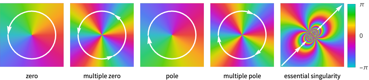
- ComplexPlot uses a cyclic color function over Arg[f] to identify features such as zeros, poles and essential singularities. The color function goes from
 to
to  counterclockwise around zeros, clockwise around poles and infinite cycles near essential singularities.
 - ComplexPlot[pred,{z,n}] is equivalent to ComplexPlot[pred,{z,-n-n I,n+n I}].
- ComplexPlot treats the variable z as local, effectively using Block.
- ComplexPlot has attribute HoldAll and evaluates f only after assigning specific numerical values to z. In some cases, it may be more efficient to use Evaluate to evaluate f symbolically first.
- No color is applied in any regions where the corresponding f evaluates to None.
- ComplexPlot has the same options as Graphics, with the following additions and changes: [List of all options]
-
Axes None whether to draw axes BoundaryStyle Automatic how to draw boundaries of regions ClippingStyle Automatic how to draw clipped regions ColorFunction Automatic how to apply coloring to curves or regions ColorFunctionScaling True whether to scale arguments to ColorFunction EvaluationMonitor None expression to evaluate at every function evaluation Exclusions Automatic x, y curves to exclude ExclusionsStyle None what to draw at excluded points or curves Frame Automatic whether to put a frame around the plot MaxRecursion Automatic the maximum number of recursive subdivisions allowed Mesh None how many mesh divisions to draw MeshFunctions Automatic how to determine the placement of mesh divisions MeshShading None how to shade regions between mesh points or lines MeshStyle Automatic the style for mesh divisions PlotLegends None legends for color gradients PlotPoints Automatic the initial number of sample points in each direction PlotRange Automatic range of values to include PlotRangeClipping True whether to clip at the plot range RegionFunction (True&) how to determine whether a point should be included WorkingPrecision MachinePrecision the precision used in internal computations PerformanceGoal $PerformanceGoal aspects of performance to try to optimize PlotTheme $PlotTheme overall theme for the plot - ColorFunction->{cfunc,sfunc} uses cfunc to generate the base color and sfunc to adjust the color to highlight features.
- Possible named settings for sfunc are:
-

Automatic automatic shading based on Abs[f] 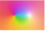
"MaxAbs" light shading of large values of Abs[f] 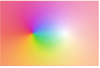
"LocalMaxAbs" light shading of an upper quantile of Abs[f] 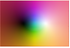
"GlobalAbs" dark to light shading of small to large values of Abs[f] 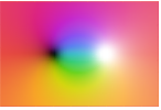
"QuantileAbs" dark to light shading based on quantiles of Abs[f] 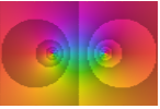
"CyclicLogAbs" cyclic dark to light shading of Log[Abs[f]] 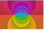
"CyclicArg" cyclic dark to light shading of Arg[f] 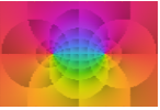
"CyclicLogAbsArg" cyclic shading of Log[Abs[f]] and Arg[f] 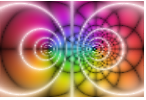
"CyclicReImLogAbs" dark cycles of Re[f] and Im[f] and light cycles of Log[Abs[f]] 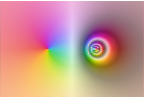
"ShiftedCyclicLogAbs" cyclic shading of Log[Abs[f]] after a threshold 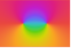
None no shading - The arguments supplied to functions in MeshFunctions and RegionFunction are
 ,
,  . Functions in ColorFunction are by default supplied with scaled versions of Re[z], Im[z], Abs[z], Arg[z], Re[f], Im[f], Abs[f], Arg[f].
List of all options
Examples
open all close allBasic Examples (3)
Plot a complex function with zeros at ![]() and poles at
and poles at ![]() :
:
ComplexPlot[(z^2 + 1/z^2 - 1), {z, -2 - 2I, 2 + 2I}]Include a legend showing how the colors vary from ![]() to
to ![]() :
:
ComplexPlot[(z^2 + 1/z^2 - 1), {z, -2 - 2I, 2 + 2I}, PlotLegends -> Automatic]Use color shading to highlight features of the function:
ComplexPlot[(z^2 + 1/z^2 - 1), {z, -2 - 2I, 2 + 2I}, ColorFunction -> "CyclicLogAbsArg"]Scope (23)
Sampling (9)
Sharp colors are obtained by using a raster image:
ComplexPlot[((z + I)^3/(z + 1)^2)Exp[(1/z - 1 - I)], {z, -2 - 2I, 2 + 2I}]Make exclusion curves smoother with PlotPoints:
ComplexPlot[z + Floor[Abs[z]], {z, -3 - 3I, 3 + 3I}, PlotPoints -> 50]Plot over an infinite domain using the standard format or a shorthand:
ComplexPlot[Sin[Sqrt[z]], {z, Infinity}]The default mesh shows curves of constant Abs[f] and Arg[f]:
ComplexPlot[z^3 - z^2 - 2, {z, -2 - 2I, 2 + 2I}, Mesh -> Automatic]Make the mesh smoother with PlotPoints:
ComplexPlot[z^3 - z^2 - 2, {z, -2 - 2I, 2 + 2I}, Mesh -> Automatic, PlotPoints -> 50]It is often convenient to use a logarithm to scale the mesh for Abs[f]:
ComplexPlot[((z + 1 + I)/1 - I + I z - z^2), {z, -2 - 2I, 2 + 2I}, Mesh -> Automatic, MeshFunctions -> {Log[Abs[#2]]&, Arg[#2]&}]Specify values for the mesh and control the style:
ComplexPlot[((z + 1 + I)/1 - I + I z - z^2), {z, -2 - 2I, 2 + 2I}, Mesh -> {Range[-1, 2, 0.1], Range[-Pi, Pi, Pi / 12]}, MeshFunctions -> {Log10[Abs[#2]]&, Arg[#2]&}, MeshStyle -> {Black, White}]Modify the mesh to show Re[f] and Im[f]:
ComplexPlot[(z^2 - I z - 1 + I/z - I), {z, -2 - 2I, 2 + 2I}, Mesh -> {Range[-4, 4, 0.25], Range[-2, 8, .25]}, MeshFunctions -> {Re[#2]&, Im[#2]&}]Emphasize branch cuts with a color scheme that is discontinuous at the cut:
ComplexPlot[1 - I + I z - z^3, {z, -5 - 5I, 5 + 5I}, ColorFunction -> "IslandColors", PlotLegends -> Automatic]Presentation (14)
ComplexPlot[(Sin[2π z]/z^3), {z, -2 - 2I, 2 + 2I}, PlotLegends -> Automatic]ComplexPlot[(z^2 + 1/z^2 - 1), {z, -2 - 2I, 2 + 2I}, Mesh -> 20, MeshFunctions -> {Log[Abs[#2]]&, Arg[#2]&}, MeshStyle -> {White, Black}]ComplexPlot[z + Floor[Abs[z]], {z, -2 - 2I, 2 + 2I}, Exclusions -> None]ComplexPlot[(z^3 - 3/z), {z, -2 - 2I, 2 + 2I}, ColorFunction -> (Hue[#8 + 0.5]&)]ComplexPlot[(z^3 - 3/z), {z, -2 - 2I, 2 + 2I}, ColorFunction -> {Automatic, None}, PlotLegends -> Automatic]Use "CyclicLogAbs" to cyclically shade colors to give the appearance of contours of constant Abs[f]:
ComplexPlot[(z^4 - 1/z^2), {z, -2 - 2I, 2 + 2I}, ColorFunction -> {Automatic, "CyclicLogAbs"}]Use "CyclicArg" to cyclically shade colors to give the appearance of contours of constant Arg[f]:
ComplexPlot[(z^4 - 1/z^2), {z, -2 - 2I, 2 + 2I}, ColorFunction -> "CyclicArg"]Use "CyclicLogAbsArg" to cyclically shade colors to give the appearance of contours of constant Abs[f] and constant Arg[f]:
ComplexPlot[(z^4 - 1/z^2), {z, -2 - 2I, 2 + 2I}, ColorFunction -> "CyclicLogAbsArg"]Use "GlobalAbs" to highlight zeros (black) and poles (white):
ComplexPlot[(z^4 - 1/z^2), {z, -2 - 2I, 2 + 2I}, ColorFunction -> "GlobalAbs"]Use "QuantileAbs" to darken small values of Abs[f] and lighten large values of Abs[f]:
ComplexPlot[(z^4 - 1/z^2), {z, -2 - 2I, 2 + 2I}, ColorFunction -> "QuantileAbs"]Use "MaxAbs" to lighten large values of Abs[f]:
ComplexPlot[(z^4 - 1/z^2), {z, -2 - 2I, 2 + 2I}, ColorFunction -> "MaxAbs"]Use "LocalMaxAbs" to lighten relatively large values of Abs[f]:
ComplexPlot[(z^4 - 1/z^2), {z, -2 - 2I, 2 + 2I}, ColorFunction -> "LocalMaxAbs"]Use "CyclicReImLogAbs" to cyclically darken based on Re[f] and Im[f] and lighten cyclically based on Log[Abs[f]]:
ComplexPlot[(z^3 - 1/z), {z, -2 - 2I, 2 + 2I}, ColorFunction -> "CyclicReImLogAbs"]Use "ShiftedCyclicLogAbs" to produce clear color wheels around zeros and cyclic contours based on Log[Abs[f]]:
ComplexPlot[(z^4 - 1/z^2), {z, -2 - 2I, 2 + 2I}, ColorFunction -> "ShiftedCyclicLogAbs"]Options (105)
AspectRatio (4)
Use Automatic to determine the ratio of the height to width for the plot:
ComplexPlot[(z + 1/z - 1), {z, -4 - 2 I, 4 + 2 I}, AspectRatio -> Automatic]Use numerical value to specify the height to width ratio:
ComplexPlot[(z + 1/z - 1), {z, -4 - 2 I, 4 + 2 I}, AspectRatio -> 1 / 2]Make the height the same as the width with AspectRatio1:
ComplexPlot[(z + 1/z - 1), {z, -4 - 2 I, 4 + 2 I}, AspectRatio -> 1]AspectRatioFull adjusts the height and width to tightly fit inside other constructs:
plot = ComplexPlot[(z + 1/z - 1), {z, -4 - 2 I, 4 + 2 I}, AspectRatio -> Full];{Framed[Pane[plot, {50, 100}]], Framed[Pane[plot, {100, 100}]], Framed[Pane[plot, {100, 50}]]}Axes (3)
By default, ComplexPlot uses a frame instead of axes:
ComplexPlot[(z + 1/z - 1), {z, -4 - 2 I, 4 + 2 I}]Use AxesTrue to draw all axes:
ComplexPlot[(z + 1/z - 1), {z, -4 - 2 I, 4 + 2 I}, Frame -> False, Axes -> True]Turn each axis on individually:
{ComplexPlot[(z + 1/z - 1), {z, -4 - 2 I, 4 + 2 I}, Frame -> False, Axes -> {True, False}], ComplexPlot[(z + 1/z - 1), {z, -4 - 2 I, 4 + 2 I}, Frame -> False, Axes -> {False, True}]}AxesLabel (3)
No axes labels are drawn by default:
ComplexPlot[(z + 1/z - 1), {z, -4 - 2 I, 4 + 2 I}, Frame -> False, Axes -> True]ComplexPlot[(z + 1/z - 1), {z, -4 - 2 I, 4 + 2 I}, Frame -> False, Axes -> True, AxesLabel -> label]ComplexPlot[(z + 1/z - 1), {z, -4 - 2 I, 4 + 2 I}, Frame -> False, Axes -> True, AxesLabel -> {"label 1", "label 2"}]AxesOrigin (2)
The position of the axes is determined automatically:
ComplexPlot[(z + 1/z - 1), {z, -4 - 2 I, 4 + 2 I}, Frame -> False, Axes -> True]Specify an explicit origin for the axes:
ComplexPlot[(z + 1/z - 1), {z, -4 - 2 I, 4 + 2 I}, Frame -> False, Axes -> True, AxesOrigin -> {2, 1}]AxesStyle (4)
Change the style for the axes:
ComplexPlot[(z + 1/z - 1), {z, -4 - 2 I, 4 + 2 I}, Frame -> False, Axes -> True, AxesStyle -> Red]Specify the style of each axis:
ComplexPlot[(z + 1/z - 1), {z, -4 - 2 I, 4 + 2 I}, Frame -> False, Axes -> True, AxesStyle -> {{Thick, Red}, {Thick, Blue}}]Use different styles for the ticks and the axes:
ComplexPlot[(z + 1/z - 1), {z, -4 - 2 I, 4 + 2 I}, Frame -> False, Axes -> True, AxesStyle -> Green, TicksStyle -> Black]Use different styles for the labels and the axes:
ComplexPlot[(z + 1/z - 1), {z, -4 - 2 I, 4 + 2 I}, Frame -> False, Axes -> True, AxesStyle -> Green, LabelStyle -> Black]ClippingStyle (3)
Clipped regions are indicated by gray by default:
ComplexPlot[z^5 + 1, {z, -2 - 2I, 2 + 2I}, PlotRange -> {0, 10}]Adjust the appearance of a clipped region:
ComplexPlot[z^5 + 1, {z, -2 - 2I, 2 + 2I}, PlotRange -> {0, 10}, ClippingStyle -> None]Color clipped regions red at the bottom and blue at the top:
ComplexPlot[z^5 + 1, {z, -2 - 2I, 2 + 2I}, PlotRange -> {0.5, 20}, ClippingStyle -> {Red, Blue}]ColorFunction (14)
Using a noncyclic color function to emphasize branch cuts:
ComplexPlot[(z^5 - 3/z^3), {z, -2 - 2I, 2 + 2I}, ColorFunction -> "GreenPinkTones", PlotLegends -> Automatic]LogGamma and Log[Gamma] have different branch cuts:
{
	ComplexPlot[LogGamma[z] , {z, -3 - 3I, 3 + 3I}, ColorFunction -> ColorData["CMYKColors"], Exclusions -> None],
	ComplexPlot[Log[Gamma[z]] , {z, -3 - 3I, 3 + 3I}, ColorFunction -> ColorData["CMYKColors"], Exclusions -> None]
	}
Specify a custom ColorFunction:
ComplexPlot[z^3 + 3z + 8 + (1/(z - 2)^2), {z, -3 - 3I, 3 + 3I}, ColorFunction -> {Hue[#8 + 0.5]&, None}, PlotLegends -> Automatic]clrs = GrayLevel /@ Join[Range[0, 1, .25], Range[.75, 0, -.25]]ComplexPlot[z^3 + 3z + 8 + (1/(z - 2)^2), {z, -3 - 3I, 3 + 3I}, ColorFunction -> {Blend[clrs, #8]&, None}, PlotLegends -> Automatic]ComplexPlot[(z^2 + 1/z^2 - 1), {z, -2 - 2I, 2 + 2I}, ColorFunction -> (Blend[{RGBColor[1, 0, 0], GrayLevel[0], RGBColor[1, 0, 0], RGBColor[1, 0.85, 0], RGBColor[1, 0, 0], GrayLevel[0], RGBColor[1, 0, 0]}, #8]&)]Color functions depend on eight arguments (Re[z], Im[z], Abs[z], Arg[z], Re[f], Im[f], Abs[f], Arg[f]):
ComplexPlot[(z^2 + 1/z^2 - 1), {z, -2 - 2I, 2 + 2I}, ColorFunction -> {Hue[(#8/2π), 0.9^#7, If[#3 < 1.5, 1, 0.75]]&, None}, ColorFunctionScaling -> False, Exclusions -> None]ComplexPlot[(z^2 + 1/z^2 - 1), {z, -2 - 2I, 2 + 2I}, ColorFunction -> {Hue[#8, 1 - Cos[8π#8]^20, 1 - 0.2SawtoothWave[6#7]]&, None}, ColorFunctionScaling -> False]ComplexPlot[z^3 - 2, {z, -2 - 2I, 2 + 2I}, ColorFunction -> {Hue[#7, 1 - 0.2SawtoothWave[8 #5], 1 - 0.2SawtoothWave[8#6]]&, None}]Color functions can be shaded to highlight features of a graph like zeros, poles and saddle points. Use "CyclicLogAbs" to cyclically shade colors to give the appearance of contours of constant Abs[f] at powers of 2:
ComplexPlot[(z^2 + 1/z^2 - 1), {z, -2 - 2I, 2 + 2I}, ColorFunction -> "CyclicLogAbs"]Use "CyclicArg" to cyclically shade colors to give the appearance of contours of constant Arg[f] at integer multiples of ![]() /6:
/6:
ComplexPlot[(z^2 + 1/z^2 - 1), {z, -2 - 2I, 2 + 2I}, ColorFunction -> "CyclicArg"]Use "CyclicLogAbsArg" shading function to combine the effects of "CyclicLogAbs" and "CyclicArg":
ComplexPlot[(z^2 + 1/z^2 - 1), {z, -2 - 2I, 2 + 2I}, ColorFunction -> "CyclicLogAbsArg"]Shading can be applied to any ColorFunction:
ComplexPlot[(z^2 + 1/z^2 - 1), {z, -2 - 2I, 2 + 2I}, ColorFunction -> {"WatermelonColors", "CyclicLogAbsArg"}]Use "GlobalAbs" to highlight zeros (black) and poles (white):
ComplexPlot[(z^2 + 1/z^2 - 1), {z, -2 - 2I, 2 + 2I}, ColorFunction -> "GlobalAbs"]Use "QuantileAbs" to lighten the image at relatively large values of Abs[f]:
ComplexPlot[(z^2 + 1/z^2 - 1), {z, -2 - 2I, 2 + 2I}, ColorFunction -> "QuantileAbs"]Use "MaxAbs" to lighten the image at large values of Abs[f]:
ComplexPlot[(z^2 + 1/z^2 - 1), {z, -2 - 2I, 2 + 2I}, ColorFunction -> "MaxAbs"]Use "LocalMaxAbs" to lighten the image at relatively large values of Abs[f]:
ComplexPlot[(z^2 + 1/z^2 - 1), {z, -2 - 2I, 2 + 2I}, ColorFunction -> "LocalMaxAbs"]Use "ShiftedCyclicLogAbs" to produce a color wheel around each zero and cyclic shading in Log[Abs[f]]:
ComplexPlot[(z^4 - 1/z^2), {z, -2 - 2I, 2 + 2I}, ColorFunction -> "ShiftedCyclicLogAbs"]Use "CyclicReImLogAbs" to darken the plot cyclically in Re[f] and Im[f] and brighten it cyclically in Log[Abs[f]]:
ComplexPlot[z^2 + 1, {z, -2 - 2I, 2 + 2I}, ColorFunction -> "CyclicReImLogAbs"]ColorFunctionScaling (1)
Exclusions (4)
Automatically determine exclusions in the modulus of the function:
ComplexPlot[z + Conjugate[z] Floor[Abs[z]], {z, -3 - 3I, 3 + 3I}]For cyclic color functions, only exclusions based on Abs[f] are shown, but for acyclic color functions, exclusions based on Arg[f] are also displayed:
ComplexPlot[z^4 - 1, {z, -2 - 2I, 2 + 2I}, ColorFunction -> "Rainbow", PlotLegends -> Automatic]Specify exclusions using equations:
ComplexPlot[z^2, {z, -3 - 3I, 3 + 3I}, Exclusions -> {Re[z] == 0}]ComplexPlot[((z + 2I)^2/(z + 2)^2), {z, -3 - 3I, 3 + 3I}, Exclusions -> {(Re[z] + 1)^2 + (Im[z] + 1)^2 == 2}]ComplexPlot[z + Conjugate[z] Floor[Abs[z]], {z, -3 - 3I, 3 + 3I}, Exclusions -> None]ExclusionsStyle (1)
Frame (4)
ComplexPlot uses a frame by default:
ComplexPlot[z ^ 3 + 3 z + 8 + 1 / (z - 2) ^ 2, {z, -3 - 3 I, 3 + 3 I}]Use FrameFalse to turn off the frame:
ComplexPlot[z ^ 3 + 3 z + 8 + 1 / (z - 2) ^ 2, {z, -3 - 3 I, 3 + 3 I}, Frame -> False]Draw a frame on the left and right edges:
ComplexPlot[z ^ 3 + 3 z + 8 + 1 / (z - 2) ^ 2, {z, -3 - 3 I, 3 + 3 I}, Frame -> {{True, True}, {False, False}}]Draw a frame on the left and bottom edges:
ComplexPlot[z ^ 3 + 3 z + 8 + 1 / (z - 2) ^ 2, {z, -3 - 3 I, 3 + 3 I}, Frame -> {{True, False}, {True, False}}]FrameLabel (4)
Place a label along the bottom frame of a plot:
ComplexPlot[z ^ 3 + 3 z + 8 + 1 / (z - 2) ^ 2, {z, -3 - 3 I, 3 + 3 I}, FrameLabel -> {"label"}]Frame labels are placed on the bottom and left frame edges by default:
ComplexPlot[z ^ 3 + 3 z + 8 + 1 / (z - 2) ^ 2, {z, -3 - 3 I, 3 + 3 I}, FrameLabel -> {"Real", "Imaginary"}]Place labels on each of the edges in the frame:
ComplexPlot[z ^ 3 + 3 z + 8 + 1 / (z - 2) ^ 2, {z, -3 - 3 I, 3 + 3 I}, FrameLabel -> {{"left", "right"}, {"bottom", "top"}}]Use a customized style for both labels and frame tick labels:
ComplexPlot[z ^ 3 + 3 z + 8 + 1 / (z - 2) ^ 2, {z, -3 - 3 I, 3 + 3 I}, FrameLabel -> {{"Imaginary", I}, {"Real", ℝ}}, LabelStyle -> Directive[Bold, StandardGray]]FrameStyle (2)
Specify the style of the frame:
ComplexPlot[z ^ 3 + 3 z + 8 + 1 / (z - 2) ^ 2, {z, -3 - 3 I, 3 + 3 I}, FrameStyle -> Directive[StandardGray, Thick]]Specify the style for each frame edge:
ComplexPlot[z ^ 3 + 3 z + 8 + 1 / (z - 2) ^ 2, {z, -3 - 3 I, 3 + 3 I}, FrameStyle -> {{Directive[Green, Thick], Directive[Red]}, {Directive[Gray, Thick], Directive[Blue]}}]FrameTicks (8)
Frame ticks are placed automatically by default:
ComplexPlot[z ^ 3 + 3 z + 8 + 1 / (z - 2) ^ 2, {z, -3 - 3 I, 3 + 3 I}]ComplexPlot[z ^ 3 + 3 z + 8 + 1 / (z - 2) ^ 2, {z, -3 - 3 I, 3 + 3 I}, FrameTicks -> None]Use frame ticks on the bottom edge:
ComplexPlot[z ^ 3 + 3 z + 8 + 1 / (z - 2) ^ 2, {z, -3 - 3 I, 3 + 3 I}, FrameTicks -> {{None, None}, {Automatic, None}}]By default, the top and right edges have tick marks but no tick labels:
ComplexPlot[z ^ 3 + 3 z + 8 + 1 / (z - 2) ^ 2, {z, -3 - 3 I, 3 + 3 I}, FrameTicks -> Automatic]Use All to include tick labels on all edges:
ComplexPlot[z ^ 3 + 3 z + 8 + 1 / (z - 2) ^ 2, {z, -3 - 3 I, 3 + 3 I}, FrameTicks -> All]Place tick marks at specific positions:
ComplexPlot[z ^ 3 + 3 z + 8 + 1 / (z - 2) ^ 2, {z, -3 - 3 I, 3 + 3 I}, Frame -> True, FrameTicks -> {{{-3, 1, 3}, {-3, 1, 3}}, {{-2, 1, 2.5}, {-2, 1, 2.5}}}]Draw frame tick marks at the specified positions with specific labels:
ComplexPlot[z ^ 3 + 3 z + 8 + 1 / (z - 2) ^ 2, {z, -3 - 3 I, 3 + 3 I}, Frame -> True, FrameTicks -> {{{{-3, -a}, {1, b}, {3, a}}, {{-3, -a}, {1, b}, {3, a}}}, {{{-2, -c}, {1, b}, {2, c}}, {{-2, -c}, {1, b}, {2, c}}}}]Specify the lengths for tick marks as a fraction of the graphics size:
ComplexPlot[z ^ 3 + 3 z + 8 + 1 / (z - 2) ^ 2, {z, -3 - 3 I, 3 + 3 I}, Frame -> True, FrameTicks -> {{Automatic, {{-2.15, -a, .4}, {0.075, b, .2}, {2.15, a, .4}}}, {Automatic, Automatic}}]Use different sizes in the positive and negative directions for each tick mark:
ComplexPlot[z ^ 3 + 3 z + 8 + 1 / (z - 2) ^ 2, {z, -3 - 3 I, 3 + 3 I}, Frame -> True, FrameTicks -> {{{{-2.15, -a, .4}, {0.075, b, .2}, {2.15, a, .4}}, {{-2.15, -a, {.4, .1}}, {0.075, b, {.2, .1}}, {2.15, a, {.4, .1}}}}, {Automatic, Automatic}}]Specify a style for each frame tick:
ComplexPlot[z ^ 3 + 3 z + 8 + 1 / (z - 2) ^ 2, {z, -3 - 3 I, 3 + 3 I}, Frame -> True, FrameTicks -> {{Automatic, {{-2.15, -a, .4, Directive[Red]}, {0.075, b, .2, Directive[Red, Thick, Dashed]}, {2.15, a, .4, Directive[Gray, Thick]}}}, {Automatic, Automatic}}]FrameTicksStyle (3)
By default, the frame ticks and frame tick labels use the same styles as the frame:
ComplexPlot[z ^ 3 + 3 z + 8 + 1 / (z - 2) ^ 2, {z, -3 - 3 I, 3 + 3 I}, FrameStyle -> Directive[Red]]Specify an overall style for the ticks, including the labels:
ComplexPlot[z ^ 3 + 3 z + 8 + 1 / (z - 2) ^ 2, {z, -3 - 3 I, 3 + 3 I}, FrameStyle -> Red, FrameTicksStyle -> Directive[Blue, Thick]]Use different styles for the different frame edges:
ComplexPlot[z ^ 3 + 3 z + 8 + 1 / (z - 2) ^ 2, {z, -3 - 3 I, 3 + 3 I}, FrameTicks -> All, FrameTicksStyle -> {{Directive[Orange, Thick], Blue}, {Red, Green}}]ImageSize (7)
Use named sizes such as Tiny, Small, Medium and Large:
{ComplexPlot[(z^2 + 1/z^2 - 1), {z, -2 - 2I, 2 + 2I}, ImageSize -> Tiny], ComplexPlot[(z^2 + 1/z^2 - 1), {z, -2 - 2I, 2 + 2I}, ImageSize -> Small]}Specify the width of the plot:
{ComplexPlot[(z^2 + 1/z^2 - 1), {z, -2 - 2I, 2 + 2I}, ImageSize -> 150], ComplexPlot[(z^2 + 1/z^2 - 1), {z, -2 - 2I, 2 + 2I}, AspectRatio -> 1.5, ImageSize -> 150]}Specify the height of the plot:
{ComplexPlot[(z^2 + 1/z^2 - 1), {z, -2 - 2I, 2 + 2I}, ImageSize -> {Automatic, 150}], ComplexPlot[(z^2 + 1/z^2 - 1), {z, -2 - 2I, 2 + 2I}, AspectRatio -> 2, ImageSize -> {Automatic, 150}]}Allow the width and height to be up to a certain size:
{ComplexPlot[(z^2 + 1/z^2 - 1), {z, -2 - 2I, 2 + 2I}, ImageSize -> UpTo[200]], ComplexPlot[(z^2 + 1/z^2 - 1), {z, -2 - 2I, 2 + 2I}, AspectRatio -> 2, ImageSize -> UpTo[200]]}Specify the width and height for a graphic, padding with space if necessary:
ComplexPlot[(z^2 + 1/z^2 - 1), {z, -2 - 2I, 2 + 2I}, ImageSize -> {200, 200}, Background -> StandardBlue]Setting AspectRatioFull will fill the available space:
ComplexPlot[(z^2 + 1/z^2 - 1), {z, -2 - 2I, 2 + 2I}, AspectRatio -> Full, ImageSize -> {200, 200}, Background -> StandardBlue]Use maximum sizes for the width and height:
{ComplexPlot[(z^2 + 1/z^2 - 1), {z, -2 - 2I, 2 + 2I}, ImageSize -> {UpTo[150], UpTo[100]}], ComplexPlot[(z^2 + 1/z^2 - 1), {z, -2 - 2I, 2 + 2I}, AspectRatio -> 2, ImageSize -> {UpTo[150], UpTo[100]}]}Use ImageSizeFull to fill the available space in an object:
Framed[Pane[ComplexPlot[(z^2 + 1/z^2 - 1), {z, -2 - 2I, 2 + 2I}, ImageSize -> Full, Background -> StandardBlue], {200, 100}]]Specify the image size as a fraction of the available space:
Framed[Pane[ComplexPlot[(z^2 + 1/z^2 - 1), {z, -2 - 2I, 2 + 2I}, AspectRatio -> Full, ImageSize -> {Scaled[0.5], Scaled[0.5]}, Background -> StandardBlue], {200, 100}]]MaxRecursion (1)
If a region function is used, MaxRecursion adapts the initial mesh:
Table[ComplexPlot[Exp[-z]Sin[3z], {z, -2 - 2I, 2 + 2I}, PlotPoints -> 5, MaxRecursion -> mr, RegionFunction -> Function[{z}, Abs[z] ≤ 2]], {mr, 0, 2}]Mesh (3)
Specify a uniform mesh in Abs[f] and Arg[f]:
ComplexPlot[z^2 + I, {z, -3 - 3I, 3 + 3I}, Mesh -> 10]Specify a different uniform mesh in each direction:
ComplexPlot[z^2 + I, {z, -3 - 3I, 3 + 3I}, Mesh -> {5, 12}]Explicitly specify the mesh values:
ComplexPlot[z^2 + I, {z, -3 - 3I, 3 + 3I}, Mesh -> {Range[0, 5, 0.5]^2, Range[-Pi, Pi, Pi / 12]}, PlotPoints -> 50]MeshFunctions (2)
Change the MeshFunctions from {Abs,Arg} to {Re,Im}:
ComplexPlot[((z^2 + I)(z^2 + 2 + 2I)/(z + 2 + I)^2), {z, -3 - 3I, 3 + 3I}, Mesh -> {Range[-5, 5], Range[-5, 5]}, MeshFunctions -> {Re[#2]&, Im[#2]&}]{![]() [
[![]() ],
],![]() } often works well in the presence of poles:
} often works well in the presence of poles:
ComplexPlot[((z^2 + I)(z^2 + 2 + 2I)/(z + 2 + I)^2), {z, -3 - 3I, 3 + 3I}, Mesh -> {40, Range[-Pi, Pi, Pi / 12]}, PlotPoints -> 100, MeshFunctions -> {Log[Abs[#2]]&, Arg[#2]&}]MeshShading (1)
MeshStyle (2)
Use a white mesh in the Re direction and a black mesh in the Im direction:
ComplexPlot[z^2 + 1, {z, -2 - 2I, 2 + 2I}, Mesh -> {Range[-10, 10, .5], Range[-10, 10, .5]}, MeshFunctions -> {Re[#2]&, Im[#2]&}, MeshStyle -> {White, Black}]Use a thick red mesh in the Abs direction and a thick blue mesh in the Arg direction:
ComplexPlot[z^2 + 1, {z, -2 - 2I, 2 + 2I}, Mesh -> {Range[0, 7], Range[-Pi, Pi, Pi / 12]}, MeshShading -> {{Gray, White}, {White, Gray}}, MeshStyle -> {Directive[Thickness[.01], Red], Directive[Thickness[.01], Blue]}]PlotLegends (2)
The Automatic legend shows the association between color and phase. The grayscale part of the legend indicates how the colors are shaded:
ComplexPlot[Sin[z], {z, -π - 2I, π + 2I}, PlotLegends -> Automatic]Cyclic shading is also reflected in the legend:
ComplexPlot[Sin[z], {z, -π - 2I, π + 2I}, ColorFunction -> "CyclicLogAbs", PlotLegends -> Automatic]PlotPoints (2)
Use more points to smooth out a nonrectangular boundary:
Table[ComplexPlot[(Sin[3z]/z^3), {z, -2 - 2I, 2 + 2I}, RegionFunction -> Function[{z}, Im[z^2] ≤ 1], PlotPoints -> i], {i, {5, 25}}]Use more points to smooth out a mesh:
Table[ComplexPlot[(Sin[3z]/z^3), {z, -2 - 2I, 2 + 2I}, Mesh -> Automatic, PlotPoints -> i], {i, {25, 75}}]PlotRange (2)
Use PlotRange to control the dimensions of the domain:
ComplexPlot[(Sin[3z]/z^3), {z, -2 - 2I, 2 + 2I}, RegionFunction -> Function[{z}, Re[z]^2 + Im[z]^2 / 4 ≤ 1], PlotRange -> {{-1, 1}, {-2, 2}}]Use PlotRange to control the range of values of Abs[f]:
ComplexPlot[(z^2 + 1/z^2 - 1), {z, -2 - 2I, 2 + 2I}, PlotRange -> {0, 5}]PlotTheme (1)
RegionFunction (3)
Use RegionFunction to adapt the shape of the region:
ComplexPlot[(z^2 + 1/z^2 - 1), {z, -2 - 2I, 2 + 2I}, RegionFunction -> Function[{z}, Abs[z] ≤ 2]]Use RegionFunction to remove zeros and poles:
ComplexPlot[(z^2 + 1/z^2 - 1), {z, -2 - 2I, 2 + 2I}, RegionFunction -> Function[{z, f}, 1 ≤ Abs[f] ≤ 2]]Shape the region based on Arg[z] or Arg[f]:
{ComplexPlot[(z^2 + 1/z^2 - 1), {z, -2 - 2I, 2 + 2I}, RegionFunction -> Function[{z, f}, -π / 2 ≤ Arg[z] < π]], ComplexPlot[(z^2 + 1/z^2 - 1), {z, -2 - 2I, 2 + 2I}, RegionFunction -> Function[{z, f}, -π / 2 ≤ Arg[f] < π]]}ScalingFunctions (4)
Domain that contains Infinity is scaled automatically:
ComplexPlot[E^-z^2 Erfc[-I z], {z, Infinity}]Use "Reverse" scale in an infinite domain:
{ComplexPlot[E^-z^2 Erfc[-I z], {z, Infinity}, ScalingFunctions -> {"Reverse", None}], ComplexPlot[E^-z^2 Erfc[-I z], {z, Infinity}, ScalingFunctions -> {None, "Reverse"}]}Use "Reciprocal" scale in an infinite domain:
ComplexPlot[E^-z^2 Erfc[-I z], {z, Infinity}, ScalingFunctions -> {"Reciprocal", None}]Use Interval to focus on a region of interest in an infinite domain:
ComplexPlot[Gamma[z], {z, Infinity}, ScalingFunctions -> {{"Infinite", Interval[{-1, 1}]}, {"Infinite", Interval[{-1, 1}]}}]Ticks (9)
Ticks are placed automatically in each plot:
ComplexPlot[z ^ 3 + 3 z + 8 + 1 / (z - 2) ^ 2, {z, -3 - 3 I, 3 + 3 I}, Frame -> False, Axes -> True]Use TicksNone to draw axes without any tick marks:
ComplexPlot[z ^ 3 + 3 z + 8 + 1 / (z - 2) ^ 2, {z, -3 - 3 I, 3 + 3 I}, Frame -> False, Axes -> True, Ticks -> None]Use ticks on the ![]() axis, but not the
axis, but not the ![]() axis:
axis:
ComplexPlot[z ^ 3 + 3 z + 8 + 1 / (z - 2) ^ 2, {z, -3 - 3 I, 3 + 3 I}, Frame -> False, Axes -> True, Ticks -> {Automatic, None}]Place tick marks at specific positions:
ComplexPlot[z ^ 3 + 3 z + 8 + 1 / (z - 2) ^ 2, {z, -3 - 3 I, 3 + 3 I}, Frame -> False, Axes -> True, Ticks -> {{-2, 1, 2.5}, {-2, 1, 2}}]Draw tick marks at the specified positions with the specified labels:
ComplexPlot[z ^ 3 + 3 z + 8 + 1 / (z - 2) ^ 2, {z, -3 - 3 I, 3 + 3 I}, Frame -> False, Axes -> True, Ticks -> {{{-2, -a}, {1, b}, {2.5, c}}, {{-2, -a}, {1, b}, {2, a}}}]Use specific ticks on one axis and automatic ticks on the other:
ComplexPlot[z ^ 3 + 3 z + 8 + 1 / (z - 2) ^ 2, {z, -3 - 3 I, 3 + 3 I}, Frame -> False, Axes -> True, Ticks -> {{{-2, -a}, {1, b}, {2.5, c}}, Automatic}]Specify the lengths for ticks as a fraction on graphics size:
ComplexPlot[z ^ 3 + 3 z + 8 + 1 / (z - 2) ^ 2, {z, -3 - 3 I, 3 + 3 I}, Frame -> False, Axes -> True, Ticks -> {{{-2, -a, .1}, {1, b, .05}, {2.5, c, .01}}, {{-2, -a, .02}, {1, b, .05}, {2, a, .1}}}]Use different sizes in the positive and negative directions for each tick:
ComplexPlot[z ^ 3 + 3 z + 8 + 1 / (z - 2) ^ 2, {z, -3 - 3 I, 3 + 3 I}, Frame -> False, Axes -> True, Ticks -> {{{-2, -a, .1}, {1, b, {.05, .05}}, {2.5, c, {.05, .1}}}, {{-2, -a, .02}, {1, b, .05}, {2, a, {.1, .1}}}}]Specify a style for each tick:
ComplexPlot[z ^ 3 + 3 z + 8 + 1 / (z - 2) ^ 2, {z, -3 - 3 I, 3 + 3 I}, Frame -> False, Axes -> True, Ticks -> {{{-2, -a, .1, Directive[Red]}, {1, b, .05, Directive[Thick, Blue]}, {2.5, c, .02, Directive[Blue]}}, {{-2, -a, .02, Directive[Thick, Red]}, {1, b, .05, Directive[Thick, Blue]}, {2, a, .1, Directive[Black]}}}]Construct a function that places ticks at the midpoint and extremes of the axis:
minMeanMax[min_, max_] := {{min, min}, {(max + min) / 2, (max + min) / 2}, {max, max}}ComplexPlot[z ^ 3 + 3 z + 8 + 1 / (z - 2) ^ 2, {z, -3 - 3 I, 3 + 4 I}, Frame -> False, Axes -> True, Ticks -> {Automatic, minMeanMax}, PlotRangePadding -> None]TicksStyle (4)
By default, the ticks and tick labels use the same styles as the axis:
ComplexPlot[z ^ 3 + 3 z + 8 + 1 / (z - 2) ^ 2, {z, -3 - 3 I, 3 + 3 I}, Frame -> False, Axes -> True, AxesStyle -> Red]Specify an overall ticks style, including the tick labels:
ComplexPlot[z ^ 3 + 3 z + 8 + 1 / (z - 2) ^ 2, {z, -3 - 3 I, 3 + 3 I}, Frame -> False, Axes -> True, TicksStyle -> Directive[Red]]Specify ticks style for each of the axes:
ComplexPlot[z ^ 3 + 3 z + 8 + 1 / (z - 2) ^ 2, {z, -3 - 3 I, 3 + 3 I}, Frame -> False, Axes -> True, TicksStyle -> {Directive[Red], Directive[Blue]}]Use a different style for the tick labels and tick marks:
ComplexPlot[z ^ 3 + 3 z + 8 + 1 / (z - 2) ^ 2, {z, -3 - 3 I, 3 + 3 I}, Frame -> False, Axes -> True, TicksStyle -> Directive[Red, Thick], LabelStyle -> Blue]WorkingPrecision (2)
Evaluate functions using machine-precision arithmetic:
ComplexPlot[Exp[I Sin[z]], {z, -2Pi - 2Pi I, 2Pi + 2Pi I}, WorkingPrecision -> MachinePrecision]Evaluate functions using arbitrary-precision arithmetic:
ComplexPlot[Exp[(5/z^4)], {z, -2 - 2 I, 2 + 2 I}, WorkingPrecision -> 5]Applications (28)
Basic Applications (7)
Make a phase portrait of a complex function ![]() . Points in the complex plane are colored (by default) by their argument, and that information is recorded in an optional legend.
. Points in the complex plane are colored (by default) by their argument, and that information is recorded in an optional legend.
The color function proceeds counterclockwise around zeros of a function:
ComplexPlot[z, {z, -2 - 2I, 2 + 2I}, PlotLegends -> Automatic]At a multiple zero, the colors cycle around the zero multiple times:
ComplexPlot[z^3, {z, -2 - 2I, 2 + 2I}, PlotLegends -> Automatic]At a pole, the colors cycle around the point in the reverse direction:
ComplexPlot[1 / z, {z, -2 - 2I, 2 + 2I}, PlotLegends -> Automatic]At an essential singularity, the colors cycle infinitely often:
ComplexPlot[Exp[I / z], {z, -0.5 - 0.5I, 0.5 + 0.5I}]At a saddle point z0 of ![]() ,
, ![]() and
and ![]() . Use "CyclicLogAbs" to highlight a saddle point that occurs at a power of 2:
. Use "CyclicLogAbs" to highlight a saddle point that occurs at a power of 2:
ComplexPlot[z^3 + 1, {z, -2 - 2I, 2 + 2I}, ColorFunction -> "CyclicLogAbs"]Or use a mesh to highlight a saddle point:
ComplexPlot[z^3 + 1, {z, -2 - 2I, 2 + 2I}, Mesh -> {Range[0, 5], Range[-Pi, Pi, Pi / 4]}, MeshFunctions -> {Log[Abs[#2]]&, Arg[#2]&}, PlotPoints -> 75]The following plot shows multiple features of the Joukowski transformation. There are simple zeros at ![]() since the colors converge at those points and cycle around the points from blue to green to red in the counterclockwise direction, consistent with the legend. Similarly, there is a simple pole at
since the colors converge at those points and cycle around the points from blue to green to red in the counterclockwise direction, consistent with the legend. Similarly, there is a simple pole at ![]() where the colors converge but cycle clockwise. There is also a saddle point at
where the colors converge but cycle clockwise. There is also a saddle point at ![]() and the branch cuts occur at the red-blue boundary:
and the branch cuts occur at the red-blue boundary:
ComplexPlot[z + (1/z), {z, -2 - 2I, 2 + 2I}, ColorFunction -> "DarkRainbow", PlotLegends -> Automatic]The following plot shows a function with simple zeros at ![]() , a double pole at
, a double pole at ![]() and a saddle point at
and a saddle point at ![]() :
:
ComplexPlot[(10(z^2 + 2z + 2)/(z - 1)^2), {z, -2 - 2I, 2 + 2I}, ColorFunction -> "CyclicLogAbs"]Other Applications (21)
General (8)
Plot complex functions of a complex variable:
ComplexPlot[Cos[z], {z, -2Pi - 3I, 2Pi + 3I}, ColorFunction -> "CyclicLogAbsArg", FrameTicks -> {{Automatic, Automatic}, {Range[-2Pi, 2Pi, Pi / 2], Automatic}}]Visualize features of a complex function of a complex variable. The following plot indicates a triple zero at ![]() , simple zeros
, simple zeros ![]() , a simple pole at
, a simple pole at ![]() , a double pole at
, a double pole at ![]() and an essential singularity at
and an essential singularity at ![]() :
:
ComplexPlot[((z + 1 + I)^3(z^2 + 1)Exp[3 / z]/(z - 1)^2(z + 1)), {z, -2 - 2I, 2 + 2I}, ColorFunction -> None]Manipulate[ComplexPlot[z^n - 1, {z, -2 - 2 I, 2 + 2 I}, Epilog -> {Circle[]}], {n, 2, 20, 1}]See the five simple real roots of ![]() in [-1,1]:
in [-1,1]:
ComplexPlot[ChebyshevT[5, z], {z, -1.2 - 1.2 I, 1.2 + 1.2 I}, ColorFunction -> "CyclicLogAbsArg"]Plots of partial sums of the geometric series suggest that the infinite series diverges for ![]() .
.
Manipulate[ComplexPlot[Sum[z^k, {k, 0, kmax}], {z, -2 - 2 I, 2 + 2 I}, ColorFunction -> "CyclicLogAbs"], {{kmax, 10, "max k"}, 1, 35, 1}]Visualize Möbius transformations:
ComplexPlot[(z - 2 + 2I/-3 + 3I - z), {z, -5 - 5 I, 5 + 5 I}, PlotPoints -> 50, Mesh -> 20, MeshStyle -> {Directive[Thick, White], Black}, MeshFunctions -> {Log[Abs[#2]]&, Arg[#2]&}, Exclusions -> None]Manipulate[
filter = ButterworthFilterModel[order, z];
ComplexPlot[Evaluate[filter[z][[1, 1]]], {z, -2 - 2I, 2 + 2I}],
{{order, 5}, 1, 20, 1}]Plot a complex function along with its Pólya field:
f = (1/z(z^2 - z - 1 - 3I));
W = Simplify[Evaluate[{1, -1}ReIm[f /. z -> x + I y]], {x∈Reals, y∈Reals}];
Show[
	ComplexPlot[Evaluate[f], {z, -2 - 2I, 2 + 2I}, Exclusions -> None],
	StreamPlot[W, {x, -2, 2}, {y, -2, 2}, StreamStyle -> White, StreamColorFunction -> None]]
Special functions (5)
ComplexPlot[Erf[z], {z, -5 - 5 I, 5 + 5 I}]ComplexPlot[(Gamma[z - I]^2/Gamma[z + I]^2), {z, -5.5 - 2I, 2 + 2I}, ColorFunction -> "ShiftedCyclicLogAbs"]A visual reminder that Log[z2]2Log[z] for Re[z]>0, but not for Re[z]<0:
{ComplexPlot[Log[z^2], {z, -2 - 2I, 2 + 2I}], ComplexPlot[2Log[z], {z, -2 - 2I, 2 + 2I}]}Visually compare a plot of a complex function with its asymptotic approximations:
f = BesselJ[3, z];
appx0 = Series[f, {z, 0, 4}]//Normal
appx∞ = Series[f, {z, ∞, 0}]//Normal{ComplexPlot[Evaluate[f], {z, -1 - I, 1 + 1 I}, PlotLabel -> TraditionalForm[f]],
ComplexPlot[Evaluate[appx0], {z, -1 - I, 1 + 1 I}, PlotLabel -> "Approximation (z ≈ 0)"]}{ComplexPlot[Evaluate[f], {z, -20 - 20 I, 20 + 20I}, PlotLabel -> TraditionalForm[f]],
ComplexPlot[Evaluate[appx∞], {z, -20 - 20 I, 20 + 20 I}, PlotLabel -> "Approximation (z ≈ ∞)"]}Observe the Hurwitz zeta function ![]() with
with ![]() over finite and infinite domains:
over finite and infinite domains:
{ComplexPlot[HurwitzZeta[10 + 4I, z], {z, -5 - 5I, 5 + 5I}, ColorFunction -> "CyclicLogAbs", PerformanceGoal -> "Speed"], ComplexPlot[HurwitzZeta[10 + 4I, z], {z, Infinity}, ColorFunction -> "CyclicLogAbs", PerformanceGoal -> "Speed"]}Observe the digamma function over finite and infinite domains:
{ComplexPlot[PolyGamma[z], {z, -5 - 5I, 5 + 5I}, ColorFunction -> "CyclicLogAbs"], ComplexPlot[PolyGamma[z], {z, Infinity}, ColorFunction -> "CyclicLogAbs"]}Analytic functions (3)
A conformal map preserves angles:
ComplexPlot[Sin[z / 2], {z, -4 - 4I, 4 + 4I}, Mesh -> 20, MeshFunctions -> {Re[#2]&, Im[#2]&}, MeshShading -> {{White, Black}, {Black, White}}]Use a mesh to illustrate a conformal map and the breakdown at ![]() where the derivative vanishes:
where the derivative vanishes:
ComplexPlot[z^2 - 2I, {z, -2 - 2I, 2 + 2I}, Mesh -> 25, MeshFunctions -> {Re[#2]&, Im[#2]&}]Compare the enhanced phase portraits of analytic and nonanalytic functions:
{ComplexPlot[(z^2 + 1/z^2 - 1), {z, -2 - 2I, 2 + 2I}, ColorFunction -> "CyclicLogAbsArg"],
	ComplexPlot[(z^2 + 1/Conjugate[z]^2 - 1), {z, -2 - 2I, 2 + 2I}, ColorFunction -> "CyclicLogAbsArg"]}
Physics (4)
Plot the field lines (black) and the potential lines (white) for two point charges of equal but opposite charge at ![]() :
:
ComplexPlot[(z + 1/z - 1), {z, -3 - 3I, 3 + 3I}, Exclusions -> None, PlotPoints -> 40, Mesh -> 30, MeshFunctions -> {Log10[Abs[#2]]&, Arg[#2]&}, MeshStyle -> {White, Black}, ColorFunction -> "GlobalAbs"]Plot the complex potential and streamlines for an ideal fluid flow exterior to a corner:
ComplexPlot[(-I z)^2 / 3 - (-z)^2 / 3, {z, -3 - 3I, 3 + 3I}, Mesh -> {Range[0, 3, .2]}, MeshFunctions -> {Im[#2]&}, RegionFunction -> Function[{z}, Arg[z] < -π / 2 || Arg[z] > 0], BoundaryStyle -> None]Plot the complex potential and streamlines for an ideal fluid flow around a cylinder:
ComplexPlot[z + (1/z) + I Log[z], {z, -2 - 2 I, 2 + 2 I}, Mesh -> {Range[-3, 3, .2]}, PlotPoints -> 75, MeshFunctions -> {Im[#2]&}, MeshStyle -> Directive[Thick, White], Epilog -> {Opacity[.25], Disk[]}, Exclusions -> None, ColorFunction -> None]Plot the complex potential and streamlines for ideal fluid flow around an elliptical cylinder with fluid speed ![]() and angle of attack
and angle of attack ![]() :
:
{a, c, α, U} = {1, 0.75, (π/6), 1};
Γ = -4Pi U a Sin[α];F1 = U z Exp[-I α] + (U a^2Exp[I α]/z) - I (Γ/2Pi)Log[z] /. z -> (z/2) + Sqrt[(z^2/4) - c^2];
F2 = U z Exp[-I α] + (U a^2Exp[I α]/z) - I (Γ/2Pi)Log[z] /. z -> (z/2) - Sqrt[(z^2/4) - c^2];Show[
ComplexPlot[F1, {z, 0 - 5 I, 5 + 5 I}, PlotPoints -> 75, Mesh -> {Range[-8, 8, .5]}, MeshFunctions -> {Im[#2]&}, MeshStyle -> Directive[Thick, White], Exclusions -> None, BoundaryStyle -> None, ColorFunction -> None],
ComplexPlot[F2, {z, -5 - 5 I, 0 + 5 I}, PlotPoints -> 75, Mesh -> {Range[-5, 8, .5]}, MeshFunctions -> {Im[#2]&}, MeshStyle -> Directive[Thick, White], Exclusions -> None, BoundaryStyle -> None, ColorFunction -> None],
Graphics[{Black, Thick, Opacity[.5], Disk[{0, 0}, {a + (c^2/a), a - (c^2/a)}]}]
, PlotRange -> 5]Transforms (1)
Plot Fourier and Laplace transforms:
ft = FourierTransform[Exp[-x^2]UnitStep[x], x, ω]ComplexPlot[ft, {ω, -10 - 10I, 10 + 0I}]lt = LaplaceTransform[t^2 SawtoothWave[t / 2], t, s]//ApartComplexPlot[lt, {s, -10 - 15I, 20 + 15I}, Exclusions -> None]Properties & Relations (8)
ComplexPlot is a special case of DensityPlot:
ComplexPlot[Log[z], {z, 3}]DensityPlot[Arg[Log[x + I y]], {x, -3, 3}, {y, -3, 3}, ColorFunction -> (Hue[(#/2Pi)]&), ColorFunctionScaling -> False]Use ComplexPlot3D to use the ![]() axis for the magnitude:
axis for the magnitude:
ComplexPlot3D[Log[z], {z, 3}]Use ComplexArrayPlot for arrays of complex numbers:
ComplexArrayPlot[Table[Table[Log[x + I y], {x, -2, 2, 0.1}], {y, -2, 2, 0.1}]]The appearance may be different from ComplexPlot depending on how the data is arranged:
ComplexArrayPlot[Reverse@Table[Table[Log[x + I y], {x, -2, 2, 0.1}], {y, -2, 2, 0.1}]]Use ReImPlot and AbsArgPlot to plot complex values over the real numbers:
ReImPlot[Log[x], {x, -3, 3}]AbsArgPlot[Log[x], {x, -3, 3}]Use ComplexListPlot to show the location of complex numbers in the plane:
ComplexListPlot[RandomComplex[{-3 - 3I, 3 + 3I}, 100]]ComplexContourPlot plots curves over the complexes:
ComplexContourPlot[Abs[Log[z]] == 1, {z, 3}]ComplexRegionPlot plots regions over the complexes:
ComplexRegionPlot[Abs[Log[z]] < 1, {z, 3}]ComplexStreamPlot and ComplexVectorPlot treat complex numbers as directions:
ComplexStreamPlot[Log[z], {z, 3}]ComplexVectorPlot[Log[z], {z, 3}]Possible Issues (2)
ComplexPlot does not do adaptive sampling:
ComplexPlot[Exp[1 / z^3 / 2], {z, -0.25 - 0.25I, 0.25 + 0.25I}]Meshes may bunch up near a pole or singular point with MeshAutomatic:
{ComplexPlot[z + 1 / z, {z, -2 - 2I, 2 + 2I}, Mesh -> Automatic, MeshFunctions -> {Re[#2]&, Im[#2]&}],
ComplexPlot[z + 1 / z, {z, -2 - 2I, 2 + 2I}, Mesh -> {Range[-2, 2, .5], Range[-2, 2, .5]}, MeshFunctions -> {Re[#2]&, Im[#2]&}]}Text
Wolfram Research (2019), ComplexPlot, Wolfram Language function, https://reference.wolfram.com/language/ref/ComplexPlot.html (updated 2021).
CMS
Wolfram Language. 2019. "ComplexPlot." Wolfram Language & System Documentation Center. Wolfram Research. Last Modified 2021. https://reference.wolfram.com/language/ref/ComplexPlot.html.
APA
Wolfram Language. (2019). ComplexPlot. Wolfram Language & System Documentation Center. Retrieved from https://reference.wolfram.com/language/ref/ComplexPlot.html