


ComplexVectorPlot
ComplexVectorPlot[f,{z,zmin,zmax}]
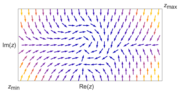
generates a vector plot of the vector field {Re[f],Im[f]} over the complex rectangle with corners zmin and zmax.
ComplexVectorPlot[{f1,f2,…},{z,zmin,zmax}]
plots several vector fields.
Details and Options
- ComplexVectorPlot is also known as field plot and direction plot.
- ComplexVectorPlot displays a vector field by drawing arrows. By default, the direction of the vector is indicated by the direction of the arrow, and the magnitude is indicated by its color.
- ComplexVectorPlot omits any arrows for which f does not evaluate to a complex number.
- ComplexVectorPlot[f,{z,n}] is equivalent to ComplexVectorPlot[f,{z,-n-n I,n+n I}].
- ComplexVectorPlot treats the variable z as local, effectively using Block.
- ComplexVectorPlot has attribute HoldAll and evaluates f only after assigning specific numerical values to z. In some cases, it may be more efficient to use Evaluate to evaluate f symbolically first.
- ComplexVectorPlot has the same options as Graphics, with the following additions and changes: [List of all options]
-
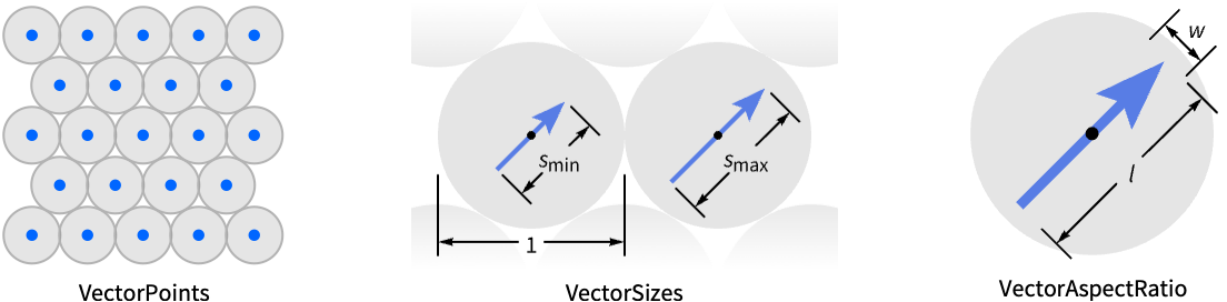
AspectRatio 1 ratio of height to width ClippingStyle Automatic how to display arrows outside the vector range EvaluationMonitor None expression to evaluate at every function evaluation Frame True whether to draw a frame around the plot FrameTicks Automatic frame tick marks Method Automatic methods to use for the plot PerformanceGoal $PerformanceGoal aspects of performance to try to optimize PlotLegends None legends to include PlotRange {Full,Full} range of x, y values to include PlotRangePadding Automatic how much to pad the range of values PlotTheme $PlotTheme overall theme for the plot RegionFunction (True&) determine what region to include RegionBoundaryStyle Automatic how to style plot region boundaries RegionFillingStyle Automatic how to style plot region interiors VectorAspectRatio Automatic width to length ratio for arrows VectorColorFunction Automatic how to color arrows VectorColorFunctionScaling True whether to scale the argument to VectorColorFunction VectorMarkers Automatic shape to use for arrows VectorPoints Automatic the number or placement of arrows VectorRange Automatic range of vector lengths to show VectorScaling None how to scale the sizes of arrows VectorSizes Automatic sizes of displayed arrows VectorStyle Automatic how to style arrows WorkingPrecision MachinePrecision precision to use in internal computations - The individual arrows are scaled to fit inside bounding circles around each point.
- VectorPoints{c1,c2,…} uses the complex numbers c1, c2, etc.… as the points at which to draw the arrows.
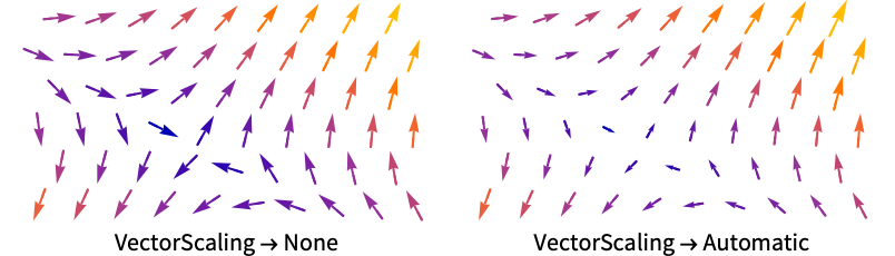
- VectorScaling scales the magnitudes of the vectors into the range of arrow sizes smin to smax given by VectorSizes.
- VectorScaling->Automatic will scale the arrow lengths depending on the vector magnitudes:
- The arrow markers given by VectorMarkers are drawn inside a box whose width and length are in the proportion
 specified by VectorAspectRatio.
 - Common markers include:
-
"Segment" line segment aligned in the field direction 
"PinDart" pin dart aligned along the field 
"Dart" dart-shaped marker 
"Drop" drop-shaped marker - VectorColorFunction->None will draw the arrows with the style specified by VectorStyle.
- The arguments supplied to functions in RegionFunction and VectorColorFunction are z and f.
List of all options
Examples
open all close allBasic Examples (3)
Plot the vector field for ![]() with color indicating the vector magnitude:
with color indicating the vector magnitude:
ComplexVectorPlot[z ^ 2, {z, -3 - 3I, 3 + 3I}]Include a legend for the vector magnitudes:
ComplexVectorPlot[z ^ 2, {z, -3 - 3I, 3 + 3I}, PlotLegends -> Automatic]Use a drop-shaped marker to represent the vectors:
ComplexVectorPlot[z ^ 2 + Sin[z], {z, 5}, VectorMarkers -> "Drop"]Scope (19)
Sampling (7)
Plot a vector field with vectors placed with specified densities:
{ComplexVectorPlot[z ^ 2 + Sin[z], {z, 5}, VectorPoints -> Coarse], ComplexVectorPlot[z ^ 2 + Sin[z], {z, 5}, VectorPoints -> Fine]}Sample the vector field on a regular grid of points:
ComplexVectorPlot[z ^ 2 + Sin[z], {z, 5}, VectorPoints -> "Regular"]Sample the vector field on an irregular mesh:
ComplexVectorPlot[z ^ 2 + Sin[z], {z, 5}, VectorPoints -> "Mesh"]Specify how many vector points to use in each direction:
ComplexVectorPlot[z ^ 2 + Sin[z], {z, 5}, VectorPoints -> 10]Plot the vectors that go through a set of seed points:
points = RandomComplex[{-5 - 5I, 5 + 5I}, 25];ComplexVectorPlot[z ^ 2 + Sin[z], {z, 5}, VectorPoints -> points, Epilog -> {Green, PointSize[Medium], Point[ReIm[points]]}]Plot vectors over a specified region:
ComplexVectorPlot[z ^ 2 + Sin[z], {z, 5}, RegionFunction -> Function[{z, f}, 1 < Abs[z] < 5]]Plot the fields for a function and its conjugate:
ComplexVectorPlot[{z, Conjugate[z]}, {z, 3}, VectorColorFunction -> None]Use Evaluate to evaluate the vector field symbolically before numeric assignment:
ComplexVectorPlot[Evaluate[D[z ^ 3, {z}]], {z, 10}]Presentation (12)
Plot a vector field with automatically scaled arrows:
ComplexVectorPlot[z Sin[z], {z, 5}, VectorScaling -> Automatic]Plot a vector field with arrows of specified size:
{ComplexVectorPlot[z Sin[z], {z, 5}, VectorSizes -> Tiny], ComplexVectorPlot[z Sin[z], {z, 5}, VectorSizes -> Large]}Draw the arrows starting from the sample points:
pts = Flatten[Table[x + I * y, {x, -3, 3}, {y, -3, 3}]];ComplexVectorPlot[I z, {z, 3}, VectorMarkers -> Placed["Arrow", "Start"], VectorPoints -> pts, Epilog -> {AbsolutePointSize[5], Green, Point[ReIm[pts]]}]Draw the arrows without the arrowheads:
ComplexVectorPlot[Sinh[z], {z, 3}, VectorMarkers -> "Segment"]Use drop-like shapes instead of arrows:
ComplexVectorPlot[Sinh[z], {z, 3}, VectorMarkers -> "Drop"]Change the overall shape of the markers:
ComplexVectorPlot[Sinh[z], {z, 3}, VectorMarkers -> "Drop", VectorAspectRatio -> 0.5]Change the default color function:
VectorPlot[{x, -y ^ 2 + x + 2}, {x, -3, 3}, {y, -3, 3}, VectorColorFunction -> "AvocadoColors"]VectorPlot[{x, -y ^ 2 + x + 2}, {x, -3, 3}, {y, -3, 3}, VectorColorFunction -> "AvocadoColors", PlotLegends -> Automatic]Vary the arrow sizes instead of the colors:
ComplexVectorPlot[z Sin[z], {z, 5}, VectorColorFunction -> None, VectorScaling -> Automatic]Set the style for multiple vector fields:
VectorPlot[{{-1 - x ^ 2 + y, 1 + x - y ^ 2}, {-(1 + x - y ^ 2), -1 - x ^ 2 + y}}, {x, -3, 3}, {y, -3, 3}, VectorColorFunction -> None, VectorMarkers -> {"Drop", "Dart"}, VectorStyle -> {Orange, Green}]ComplexVectorPlot[z Sin[z], {z, 5}, VectorColorFunction -> None, VectorStyle -> Directive[Orange, Dashed]]Set the style for multiple vector fields:
ComplexVectorPlot[{z, z ^ 2}, {z, 5}, PlotLegends -> {"one", "two"}, VectorColorFunction -> None, VectorStyle -> {Orange, Green}]Use a theme with simple ticks and grid lines:
ComplexVectorPlot[z Sin[z], {z, 5}, PlotTheme -> "Business"]Options (65)
Background (1)
ClippingStyle (4)
By default, extremely short and extremely long vectors are displayed:
ComplexVectorPlot[(z + 1/Abs[z + 1]^3) - (z - 1/Abs[z - 1]^3), {z, -3 - 3I, 3 + 3I}, VectorRange -> {0.1, 2}]Use ClippingStyleNone to remove extreme vectors from the plot:
ComplexVectorPlot[(z + 1/Abs[z + 1]^3) - (z - 1/Abs[z - 1]^3), {z, -3 - 3I, 3 + 3I}, VectorRange -> {0.1, 2}, ClippingStyle -> None]ComplexVectorPlot[(z + 1/Abs[z + 1]^3) - (z - 1/Abs[z - 1]^3), {z, -3 - 3I, 3 + 3I}, VectorRange -> {0.1, 2}, ClippingStyle -> Red]Style the short and long clipped vectors differently:
ComplexVectorPlot[(z + 1/Abs[z + 1]^3) - (z - 1/Abs[z - 1]^3), {z, -3 - 3I, 3 + 3I}, VectorRange -> {0.1, 2}, ClippingStyle -> {Red, Green}]EvaluationMonitor (2)
Show where the vector field function is sampled:
ComplexListPlot[Reap[ComplexVectorPlot[I z, {z, -2 - 2I, 2 + 2I}, EvaluationMonitor :> Sow[z]]][[-1, 1]]]Count the number of times the vector field function is evaluated:
Block[{k = 0}, ComplexVectorPlot[I z, {z, -2 - 2I, 2 + 2I}, EvaluationMonitor :> k++];k]PlotLegends (5)
Include a legend for the vector norms:
ComplexVectorPlot[z, {z, -2 - 2I, 2 + 2I}, PlotLegends -> Automatic]Use the expressions in the legend for multiple vector functions:
ComplexVectorPlot[{z, I z}, {z, -2 - 2I, 2 + 2I}, PlotLegends -> "Expressions", VectorColorFunction -> None]Specify the legend labels for multiple functions:
ComplexVectorPlot[{z, I z}, {z, -2 - 2I, 2 + 2I}, PlotLegends -> {"one", "two"}, VectorColorFunction -> None]Control the placement of the legend:
ComplexVectorPlot[{z, I z}, {z, -2 - 2I, 2 + 2I}, PlotLegends -> Placed[{"one", "two"}, Below], VectorColorFunction -> None]Use a legend with placeholders:
ComplexVectorPlot[{z, I z}, {z, -2 - 2I, 2 + 2I}, PlotLegends -> Automatic, VectorColorFunction -> None]PlotRange (5)
The full plot range is used by default:
ComplexVectorPlot[z - Conjugate[z], {z, -5 - 5I, 5 + 5I}]Specify an explicit limit for both real and imaginary ranges:
ComplexVectorPlot[z - Conjugate[z], {z, -5 - 5I, 5 + 5I}, PlotRange -> 7]Specify an explicit real range:
ComplexVectorPlot[z - Conjugate[z], {z, -5 - 5I, 5 + 5I}, PlotRange -> {{-3, 5}, Automatic}]Specify an explicit imaginary range:
ComplexVectorPlot[z - Conjugate[z], {z, -5 - 5I, 5 + 5I}, PlotRange -> {-3, 5}]Specify different real and imaginary ranges:
ComplexVectorPlot[z - Conjugate[z], {z, -5 - 5I, 5 + 5I}, PlotRange -> {{0, Full}, {-3, 5}}]PlotTheme (2)
RegionBoundaryStyle (5)
Show the region defined by a region function:
ComplexVectorPlot[I z, {z, -2 - 2I, 2 + 2I}, RegionFunction -> Function[{z, f}, Abs[z] < 2]]The boundaries of full rectangular regions are not shown:
ComplexVectorPlot[I z, {z, -2 - 2I, 2 + 2I}]Use None to not show the boundary:
ComplexVectorPlot[I z, {z, -2 - 2I, 2 + 2I}, RegionFunction -> Function[{z, f}, Abs[z] < 2], RegionBoundaryStyle -> None]Omit the interior filling as well:
ComplexVectorPlot[I z, {z, -2 - 2I, 2 + 2I}, RegionFunction -> Function[{z, f}, Abs[z] < 2], RegionBoundaryStyle -> None, RegionFillingStyle -> None]Specify a style for the boundary:
ComplexVectorPlot[I z, {z, -2 - 2I, 2 + 2I}, RegionFunction -> Function[{z, f}, Abs[z] < 2], RegionBoundaryStyle -> Red]Specify a style for full rectangular regions:
ComplexVectorPlot[I z, {z, -2 - 2I, 2 + 2I}, RegionBoundaryStyle -> Red]RegionFillingStyle (5)
Show the region defined by a region function:
ComplexVectorPlot[I z, {z, -2 - 2I, 2 + 2I}, RegionFunction -> Function[{z, f}, Abs[z] < 2]]The interiors of full rectangular regions are not shown:
ComplexVectorPlot[I z, {z, -2 - 2I, 2 + 2I}]Use None to not show the interior filling:
ComplexVectorPlot[I z, {z, -2 - 2I, 2 + 2I}, RegionFunction -> Function[{z, f}, Abs[z] < 2], RegionFillingStyle -> None]Omit the boundary curve as well:
ComplexVectorPlot[I z, {z, -2 - 2I, 2 + 2I}, RegionFunction -> Function[{z, f}, Abs[z] < 2], RegionFillingStyle -> None, RegionBoundaryStyle -> None]Specify a style for the interior filling:
ComplexVectorPlot[I z, {z, -2 - 2I, 2 + 2I}, RegionFunction -> Function[{z, f}, Abs[z] < 2], RegionFillingStyle -> Gray]Specify a style for full rectangular region:
ComplexVectorPlot[I z, {z, -2 - 2I, 2 + 2I}, RegionFillingStyle -> Gray]RegionFunction (2)
Restrict the plotting region based on ![]() :
:
ComplexVectorPlot[z^2 + 1, {z, -3 - 3I, 3 + 3I}, RegionFunction -> Function[{z, f}, Abs[z] ≥ 1]]Restrict the plotting region based on ![]() :
:
ComplexVectorPlot[z^2 + 1, {z, -3 - 3I, 3 + 3I}, RegionFunction -> Function[{z, f}, Abs[f] ≥ 4]]VectorAspectRatio (2)
The default ratio of the width to the length of the vector marker is 1/4:
ComplexVectorPlot[(1/z^2 + 1), {z, -3 - 3I, 3 + 3I}]Modify the ratio of the width to the length of the vector marker:
Table[ComplexVectorPlot[(1/z^2 + 1), {z, -3 - 3I, 3 + 3I}, VectorAspectRatio -> var, PlotLabel -> var], {var, {1 / 4, 1 / 2}}]VectorColorFunction (5)
Vectors are colored according to their norms by default:
ComplexVectorPlot[ArcSin[z], {z, -3 - 3I, 3 + 3I}]Choose the color scheme for coloring vectors by their norms:
ComplexVectorPlot[ArcSin[z], {z, -3 - 3I, 3 + 3I}, VectorColorFunction -> Hue]Use any named color gradient from ColorData:
ComplexVectorPlot[ArcSin[z], {z, -3 - 3I, 3 + 3I}, VectorColorFunction -> "Rainbow"]Color the vectors according to the real part of its location:
ComplexVectorPlot[ArcSin[z], {z, -3 - 3I, 3 + 3I}, VectorColorFunction -> Function[{z, f}, ColorData["ThermometerColors"][Re[z]]]]Color the vectors according to the real part of the function:
ComplexVectorPlot[ArcSin[z], {z, -3 - 3I, 3 + 3I}, VectorColorFunction -> Function[{z, f}, ColorData["ThermometerColors"][Re[f]]]]VectorColorFunctionScaling (2)
By default, scaled values are used:
ComplexVectorPlot[ArcSin[z], {z, -3 - 3I, 3 + 3I}, VectorColorFunction -> Hue]Use VectorColorFunctionScalingFalse to get unscaled values:
ComplexVectorPlot[ArcSin[z], {z, -3 - 3I, 3 + 3I}, VectorColorFunction -> Hue, VectorColorFunctionScaling -> False]VectorMarkers (4)
Vectors are drawn as arrows by default:
ComplexVectorPlot[z Log[z], {z, -3 - 3I, 3 + 3I}]Use a named appearance to draw the vectors:
plotmarkers = {"Arrow", "ArrowArrow", "BackwardPointer", "BarDot", "Box", "Circle", "CircleArrow", "Dart", "Disk", "Dot", "DotArrow", "DotDot", "DoubleDart", "Drop", "Paddle", "PinDart", "Pointer", "Segment", "Spindle", "Toothpick"};Manipulate[ComplexVectorPlot[z Log[z], {z, -3 - 3I, 3 + 3I}, VectorMarkers -> m, PlotLabel -> m], {m, plotmarkers}]Use different markers for different vector fields:
ComplexVectorPlot[{z Log[z], z}, {z, -3 - 3I, 3 + 3I}, VectorMarkers -> {"Drop", "Dart"}]By default, markers are centered on vector points:
pts = Join@@Table[x + I y, {x, -3, 3}, {y, -3, 3}];ComplexVectorPlot[z Log[z], {z, -3 - 3I, 3 + 3I}, VectorMarkers -> "Arrow", VectorPoints -> pts, Epilog -> {Red, Point[ReIm[pts]]}]Start the vectors at the points:
ComplexVectorPlot[z Log[z], {z, -3 - 3I, 3 + 3I}, VectorMarkers -> Placed["Arrow", "Start"], VectorPoints -> pts, Epilog -> {Red, Point[ReIm[pts]]}]End the vectors at the points:
ComplexVectorPlot[z Log[z], {z, -3 - 3I, 3 + 3I}, VectorMarkers -> Placed["Arrow", "End"], VectorPoints -> pts, Epilog -> {Red, Point[ReIm[pts]]}]VectorPoints (5)
Use automatically determined vector points:
ComplexVectorPlot[Exp[Sqrt[z]], {z, -3 - 3I, 3 + 3I}]Use symbolic names to specify the set of field vectors:
Table[ComplexVectorPlot[Exp[Sqrt[z]], {z, -3 - 3I, 3 + 3I}, PlotLabel -> k, VectorPoints -> k], {k, {Fine, Automatic, Coarse}}]Create a hexagonal grid of field vectors with the same number of arrows in the real and imaginary directions:
ComplexVectorPlot[Exp[Sqrt[z]], {z, -3 - 3I, 3 + 3I}, VectorPoints -> 5]Create a hexagonal grid of field vectors with a different number of arrows in the real and imaginary directions:
ComplexVectorPlot[Exp[Sqrt[z]], {z, -3 - 3I, 3 + 3I}, VectorPoints -> {4, 7}]Specify a list of points for showing field vectors:
ComplexVectorPlot[Exp[Sqrt[z]], {z, -3 - 3I, 3 + 3I}, VectorPoints -> RandomComplex[{-3 - 3I, 3 + 3I}, 300]]VectorRange (6)
By default, vector ranges are determined automatically:
ComplexVectorPlot[(z/Abs[z]^3), {z, -3 - 3I, 3 + 3I}, PlotLegends -> Automatic]Plot vectors with magnitudes between 0.2 and 2:
ComplexVectorPlot[(z/Abs[z]^3), {z, -3 - 3I, 3 + 3I}, PlotLegends -> Automatic, VectorRange -> {0.2, 2}, ClippingStyle -> None]Plot vectors with magnitudes between 0.2 and 2 with scaled arrow lengths:
ComplexVectorPlot[(z/Abs[z]^3), {z, -3 - 3I, 3 + 3I}, PlotLegends -> Automatic, VectorRange -> {0.2, 2}, ClippingStyle -> None, VectorScaling -> Automatic]ComplexVectorPlot[(z/Abs[z]^3), {z, -3 - 3I, 3 + 3I}, PlotLegends -> Automatic, VectorRange -> {0.2, 10}, ClippingStyle -> Red]Plot scaled vectors with all lengths:
ComplexVectorPlot[(z/Abs[z]^3), {z, -3 - 3I, 3 + 3I}, PlotLegends -> Automatic, VectorRange -> All, VectorScaling -> Automatic]Increase the lengths of the smaller vectors:
ComplexVectorPlot[(z/Abs[z]^3), {z, -3 - 3I, 3 + 3I}, PlotLegends -> Automatic, VectorRange -> All, VectorScaling -> Automatic, VectorSizes -> {0.5, 1}]VectorScaling (2)
By default, VectorScaling is None:
ComplexVectorPlot[Sqrt[Sin[z]], {z, -3 - 3I, 3 + 3I}, VectorScaling -> None]Use automatic scaling to scale the length of vectors:
ComplexVectorPlot[Sqrt[Sin[z]], {z, -3 - 3I, 3 + 3I}, VectorScaling -> Automatic]VectorSizes (2)
Vector markers have automatically scaled lengths to prevent any vectors from being too small and to keep them from overlapping:
ComplexVectorPlot[(z + 1/Abs[z + 1]^3) - (z - 1/Abs[z - 1]^3), {z, -3 - 3I, 3 + 3I}, VectorMarkers -> "Circle", VectorScaling -> Automatic]Specify a minimum and maximum scaled vector size:
ComplexVectorPlot[(z + 1/Abs[z + 1]^3) - (z - 1/Abs[z - 1]^3), {z, -3 - 3I, 3 + 3I}, VectorMarkers -> "Circle", VectorSizes -> {0, 1}, VectorScaling -> Automatic]VectorStyle (6)
Set the style for the displayed vectors:
ComplexVectorPlot[z Log[Sin[z]], {z, -3 - 3I, 3 + 3I}, VectorStyle -> Red, VectorColorFunction -> None]Set the style for multiple functions:
ComplexVectorPlot[{z Log[Sin[z]], z}, {z, -3 - 3I, 3 + 3I}, VectorStyle -> {Red, Blue}, VectorColorFunction -> None]Use Arrowheads to specify an explicit style of the arrowheads:
ComplexVectorPlot[z Log[Sin[z]], {z, -3 - 3I, 3 + 3I}, VectorPoints -> 8, PlotRange -> All, VectorStyle -> Arrowheads[{{0.03, Automatic, Graphics[Circle[]]}}]]Specify both arrow tail and head:
ComplexVectorPlot[z Log[Sin[z]], {z, -3 - 3I, 3 + 3I}, VectorPoints -> 8, PlotRange -> All, VectorStyle -> Arrowheads[{{0.03, Automatic, Graphics[Rectangle[{-0.5, -0.5}, {0.5, 0.5}]]}, {0.03, Automatic, Graphics[Circle[]]}}]]Graphics primitives without Arrowheads are scaled based on the vector scale:
ComplexVectorPlot[z Log[Sin[z]], {z, -3 - 3I, 3 + 3I}, VectorPoints -> 8, PlotRange -> All, VectorStyle -> Graphics[Circle[]]]Change the scaling using the VectorScaling option:
ComplexVectorPlot[z Log[Sin[z]], {z, -3 - 3I, 3 + 3I}, VectorPoints -> 8, PlotRange -> All, VectorStyle -> Graphics[Circle[]], VectorScaling -> Automatic]Applications (7)
For a complex function f, plot {Re[f],Im[f]}:
ComplexVectorPlot[z Log[2z] + 3 , {z, -2 - 2 I, 2 + 2 I}]The vector length increases with Abs[f] and the orientation is determined by Arg[f]:
Show[ComplexPlot[z Log[2z] + 3, {z, -2 - 2 I, 2 + 2 I}, PlotLegends -> Automatic], ComplexVectorPlot[z Log[2z] + 3 , {z, -2 - 2 I, 2 + 2 I}, VectorStyle -> Black, VectorColorFunction -> None]]Identify poles and zeros. Poles are visible at ![]() and
and ![]() :
:
ComplexVectorPlot[(1/(z - 3) (z^2 + 4)) , {z, -4 - 4 I, 4 + 4 I}]The zeros at ![]() and
and ![]() are more readily visible if the vectors are scaled:
are more readily visible if the vectors are scaled:
ComplexVectorPlot[(z - 3) (z^2 + 4) , {z, -4 - 4 I, 4 + 4 I}, VectorScaling -> Automatic]Vectors in the field rotate twice along the unit circle surrounding the zero of the function ![]() at the origin, which implies that
at the origin, which implies that ![]() has a double zero at the origin:
has a double zero at the origin:
pts = N@Table[ReIm[Exp[I t]], {t, 0, 2π, (π/12)}];
ComplexVectorPlot[z Sin[z], {z, -2 - 2 I, 2 + 2 I}, VectorPoints -> pts, Epilog -> Circle[], PlotRangePadding -> Scaled[0.1]]reim = Simplify[ReIm[ComplexExpand[z Sin[z] /. z -> x + I y]], {x∈Reals, y∈Reals}];
arrow = Arrow[{{x, y}, {x, y} + reim} /. {x -> Cos[t], y -> Sin[t]}];With[{arrow = arrow}, Manipulate[
Show[
ComplexPlot[z Sin[z], {z, -2 - 2 I, 2 + 2 I}, Epilog -> {Circle[], arrow}],
ComplexVectorPlot[z Sin[z], {z, -2 - 2 I, 2 + 2 I}, VectorStyle -> Black]
],
{t, 0, 2π}]
]The function ![]() has a pole of order 2 at
has a pole of order 2 at ![]() since
since ![]() has a double zero:
has a double zero:
f[z_] := z^2 + 1pts = N@Table[ReIm[Exp[I t]], {t, 0, 2π, (π/25)}];
ComplexVectorPlot[f[(1/z)] , {z, -1 - I, 1 + I}, VectorPoints -> pts, VectorScaling -> None, Epilog -> Circle[], PlotRangePadding -> Scaled[0.1], VectorSizes -> {0, 1.5}]Specify a direction field and several solutions for the complex initial value problem ![]() ,
, ![]() :
:
ComplexVectorPlot[z^2, {z, -2 - 2 I, 2 + 2 I}, StreamPoints -> 20]The Pólya field of an analytic function is both divergence and curl free:
ComplexVectorPlot[Conjugate[z^2], {z, -2 - 2 I, 2 + 2 I}, VectorScaling -> Automatic]polyaField = ComplexExpand[ReIm[Conjugate[z^2] /. z -> x + I y]]
Div[polyaField, {x, y}]
Curl[polyaField, {x, y}]Examine partial sums of an infinite series:
partialSum = Sum[n(z - 1)^n, {n, 1, nmax}];
tb = Table[ComplexVectorPlot[Evaluate[partialSum], {z, -1.5I, 3 + 1.5I}, VectorRange -> {0.1, 100}, ClippingStyle -> None], {nmax, 1, 20, 1}];ListAnimate[tb]Properties & Relations (15)
ComplexVectorPlot is a special case of VectorPlot:
{ComplexVectorPlot[Sin[z], {z, 4}], VectorPlot[ReIm[Sin[x + I * y]], {x, -4 , 4}, {y, -4, 4}]}ComplexStreamPlot plots complex numbers as streamlines:
ComplexStreamPlot[Log[z], {z, 3}]ComplexStreamPlot is a special case of StreamPlot:
StreamPlot[ReIm[Log[x + I y]], {x, -3, 3}, {y, -3, 3}]Use VectorDisplacementPlot to visualize the effect of a complex function on a specified region:
VectorDisplacementPlot[ReIm[Sin[x + I y]], {x, y}∈Annulus[], VectorPoints -> Automatic, VectorSizes -> Full]Use VectorPlot3D and StreamPlot3D to visualize 3D vector fields:
{VectorPlot3D[{z, x, y}, {x, -1, 1}, {y, -1, 1}, {z, -1, 1}], StreamPlot3D[{z, x, y}, {x, -1, 1}, {y, -1, 1}, {z, -1, 1}]}ComplexContourPlot plots curves over the complexes:
ComplexContourPlot[Abs[Log[z]] == 1, {z, 3}]ComplexRegionPlot plots regions over the complexes:
ComplexRegionPlot[Abs[Log[z]] < 1, {z, 3}]ComplexPlot shows the argument and magnitude of a function using color:
ComplexPlot[Log[z], {z, 3}]Use ComplexPlot3D to use the ![]() axis for the magnitude:
axis for the magnitude:
ComplexPlot3D[Log[z], {z, 3}]Use ComplexArrayPlot for arrays of complex numbers:
ComplexArrayPlot[Table[x ^ 3 + I y ^ 2, {x, -2, 2, 0.1}, {y, -2, 2, 0.1}]]Use ReImPlot and AbsArgPlot to plot complex values over the real numbers:
ReImPlot[Log[x], {x, -3, 3}]AbsArgPlot[Log[x], {x, -3, 3}]Use ComplexListPlot to show the location of complex numbers in the plane:
ComplexListPlot[RandomComplex[{-3 - 3I, 3 + 3I}, 100]]Use ListVectorPlot for plotting data:
data = Table[ReIm[(x + I y)^2], {x, -3, 3, 0.2}, {y, -3, 3, 0.2}];ListVectorPlot[data]Use ListStreamPlot to plot streams instead of vectors:
ListStreamPlot[data]Use VectorDensityPlot to add a density plot of a scalar field:
VectorDensityPlot[ReIm[(x + I y)^2], {x, -3, 3}, {y, -3, 3}]Use StreamDensityPlot to use streams instead of vectors:
StreamDensityPlot[ReIm[(x + I y)^2], {x, -3, 3}, {y, -3, 3}]Use ListVectorDensityPlot to generate a density plot of a scalar field based on data:
data = Table[{{x, y}, ReIm[(x + I y)^2 + 1]}, {x, -3, 3, 0.2}, {y, -3, 3, 0.2}];ListVectorDensityPlot[data]Use ListStreamDensityPlot to plot streams instead of vectors:
ListStreamDensityPlot[data]Use LineIntegralConvolutionPlot to plot the line integral convolution of a vector field:
LineIntegralConvolutionPlot[ReIm[(x + I y)^3], {x, -3, 3}, {y, -3, 3}]Text
Wolfram Research (2020), ComplexVectorPlot, Wolfram Language function, https://reference.wolfram.com/language/ref/ComplexVectorPlot.html.
CMS
Wolfram Language. 2020. "ComplexVectorPlot." Wolfram Language & System Documentation Center. Wolfram Research. https://reference.wolfram.com/language/ref/ComplexVectorPlot.html.
APA
Wolfram Language. (2020). ComplexVectorPlot. Wolfram Language & System Documentation Center. Retrieved from https://reference.wolfram.com/language/ref/ComplexVectorPlot.html