


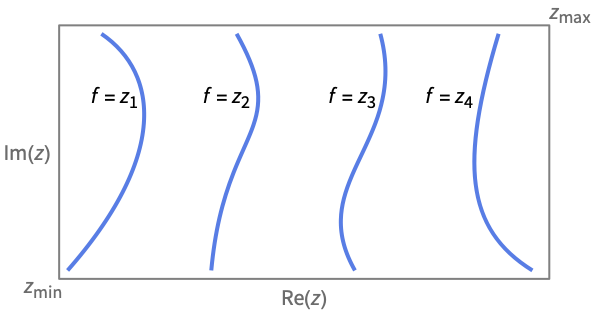
ComplexContourPlot
ComplexContourPlot[f,{z,zmin,zmax}]
generates a filled contour plot of f as a function of z.
ComplexContourPlot[{f1,f2,…},{z,zmin,zmax}]
generates contour lines for f1, f2, ….
ComplexContourPlot[f==g,{z,zmin,zmax}]
plots contour lines for which f=g.
ComplexContourPlot[{f1==g1,f2==g2,…},{z,zmin,zmax}]
plots contour lines for each of f1g1, f2=g2, ….
Details and Options
- At positions where f does not evaluate to a real number, holes are left so that the background to the contour plot shows through. The functions f and g will typically involve functions like Re, Im, Abs and Arg that extract real components from complex numbers for comparison purposes.
- ComplexContourPlot[f,{z,n}] is equivalent to ComplexContourPlot[f,{z,-n-n I,n+n I}].
- ComplexContourPlot treats the variable z as local, effectively using Block.
- ComplexContourPlot has attribute HoldAll and evaluates the fi and gi only after assigning specific numerical values to z. In some cases, it may be more efficient to use Evaluate to evaluate f and g symbolically first.
- ComplexContourPlot has the same options as Graphics, with the following additions and changes: [List of all options]
-
AspectRatio 1 ratio of height to width BoundaryStyle None how to draw RegionFunction boundaries BoxRatios Automatic effective 3D bounding-box ratios ClippingStyle None how to draw values clipped by PlotRange ColorFunction Automatic how to color regions between contour lines ColorFunctionScaling True whether to scale the argument to ColorFunction ContourLabels Automatic how to label contour levels Contours Automatic how many or what contours to use ContourShading Automatic how to shade regions between contours ContourStyle Automatic the style for contour lines EvaluationMonitor None expression to evaluate at every function evaluation Exclusions Automatic x,y curves to exclude ExclusionsStyle None what to draw at excluded curves Frame True whether to put a frame around the plot FrameTicks Automatic frame tick marks LightingAngle None effective angle of the simulated light source MaxRecursion Automatic the maximum number of recursive subdivisions allowed Mesh None how many mesh lines in each direction to draw MeshFunctions {} how to determine the placement of mesh lines MeshStyle Automatic the style for mesh lines Method Automatic the method to use for refining contours PerformanceGoal $PerformanceGoal aspects of performance to try to optimize PlotLegends None legends for contour regions PlotPoints Automatic the initial number of sample points in each direction PlotRange {Full,Full,Automatic} the range of f or other values to include PlotRangeClipping True whether to clip at the plot range PlotRangePadding Automatic how much to pad the range of values PlotTheme $PlotTheme overall theme for the plot RegionFunction (True&) how to determine whether a point should be included ScalingFunctions None how to scale individual coordinates WorkingPrecision MachinePrecision the precision used in internal computations - Typical settings for PlotLegends include:
-
None no legend Automatic automatically determine legend Placed[lspec,…] specify placement for legend - With the default setting ContourShading->Automatic, shading is used for ComplexContourPlot[f,…] but not for ComplexContourPlot[f=g,…] or ComplexContourPlot[{f1,f2,…},…].
- ComplexContourPlot[{f1==g1,f2==g2,…},…] superimposes the contour lines associated with all of the equalities fi==gi.
- In determining how to color regions between contour levels, ComplexContourPlot looks first at any explicit setting given for ContourShading, then at the setting for ColorFunction.
- When plotting contours of multiple functions ComplexContourPlot[{f1,f2,…},…], a list of contour specifications Contours{spec1,spec2,…} will use the corresponding speci for each of the fi.
- ColorData["DefaultPlotColors"] gives the default sequence of colors used by ContourStyle.
- ComplexContourPlot initially evaluates f at a grid of equally spaced sample points specified by PlotPoints. Then it uses an adaptive algorithm to subdivide at most MaxRecursion times to generate smooth contours.
- You should realize that since it uses only a finite number of sample points, it is possible for ComplexContourPlot to miss features of your functions. To check your results, you should try increasing the settings for PlotPoints and MaxRecursion.
- With some settings for PerformanceGoal, other specific option settings may be overridden.
- The arguments supplied to functions in MeshFunctions and RegionFunction are z, f.
- ColorFunction is supplied with a single argument, given by default by the average of the scaled values of f for each pair of successive contour levels.
- With the default settings Exclusions->Automatic and ExclusionsStyle->None, ComplexContourPlot breaks continuity in its sampling at any discontinuity curve it detects. The discontinuity is immediately visible only if it jumps out of a particular contour level.
- Possible settings for ScalingFunctions include:
-
sf scale the f values {sRe,sIm} scale the real and imaginary axes {sRe,sIm,sf} scale the real and imaginary axes and f values
List of all options
Examples
open all close allBasic Examples (4)
Plot a contour map of a real function of a complex variable:
ComplexContourPlot[Abs[z], {z, -3 - 3I, 3 + 3I}]Plot an equality over the complex plane:
ComplexContourPlot[Re[z] == Im[1 / z], {z, 2}]ComplexContourPlot[{Re[z], Im[1 / z]}, {z, 2}]ComplexContourPlot[{Abs[z] == Re[z] + 1, Abs[z] == Re[z] + 2, Abs[z] == Re[z] + 3}, {z, -3 - 3I, 3 + 3I}, PlotLegends -> "Expressions"]Scope (18)
Sampling (6)
More points are sampled where the function changes quickly:
ComplexContourPlot[Abs[z^2 + 1], {z, 0, 2 + 2I}, Mesh -> All]The white regions indicate where the function has been clipped. The plot range is selected automatically:
ComplexContourPlot[Abs[1 / z], {z, -3 - 3I, 3 + 3I}]Use PlotRange to focus in on areas of interest:
ComplexContourPlot[Abs[1 / z], {z, -3 - 3I, 3 + 3I}, PlotRange -> {0.2, 5}]Use PlotPoints and MaxRecursion to control adaptive sampling:
Table[ComplexContourPlot[Abs[Sin[z^1 / 2] + 1], {z, 0, 2 + 2I}, PlotPoints -> pp, MaxRecursion -> mr], {mr, {0, 2}}, {pp, {5, 15}}]Use RegionFunction to restrict the surface to a region given by inequalities:
ComplexContourPlot[Re[ArcSin[z]], {z, -3 - 3I, 3 + 3I}, RegionFunction -> Function[{z, f}, Abs[z] < 3]]Use Exclusions to control whether and where to cut for discontinuities:
{ComplexContourPlot[Arg[ArcSin[z^2]], {z, -3 - 3I, 3 + 3I}],
	ComplexContourPlot[Arg[ArcSin[z^2]], {z, -3 - 3I, 3 + 3I}, Exclusions -> None]}
Labeling and Legending (6)
Add labels for the frame and the overall plot:
ComplexContourPlot[Re[Sqrt[z]], {z, -3 - 3I, 3 + 3I}, FrameLabel -> {Re[z], Im[z]}, PlotLabel -> Re[Sqrt[z]]]ComplexContourPlot[Re[Sqrt[z]] == 1, {z, -3 - 3I, 3 + 3I}, FrameLabel -> {Re[z], Im[z]}, PlotLabel -> Re[Sqrt[z]] == 1]ComplexContourPlot[Re[Sqrt[z]], {z, -3 - 3I, 3 + 3I}, ContourLabels -> True]ComplexContourPlot[Re[Sqrt[z]], {z, -3 - 3I, 3 + 3I}, PlotLegends -> Automatic]For multiple functions, use a line legend:
ComplexContourPlot[ReIm[Sqrt[z]], {z, -3 - 3I, 3 + 3I}, PlotLegends -> "Expressions"]For multiple functions, use a line legend with placeholders:
ComplexContourPlot[ReIm[Sqrt[z]], {z, -3 - 3I, 3 + 3I}, PlotLegends -> Automatic]Add a legend for implicit curves:
ComplexContourPlot[{Re[z^2] == 1, Im[z^2] == 1}, {z, -3 - 3I, 3 + 3I}, PlotLegends -> "Expressions"]Presentation (6)
ComplexContourPlot[Re[Sqrt[z]], {z, -3 - 3I, 3 + 3I}, ColorFunction -> "Rainbow"]Use specific colors between contours:
ComplexContourPlot[Re[z^2], {z, -3 - 3I, 3 + 3I}, ContourShading -> Hue /@ Range[0, 1, 0.1]]Use different styles for the contours:
ComplexContourPlot[Re[z^2], {z, -3 - 3I, 3 + 3I}, ContourStyle -> {Red, Directive[Red, Dashed]}]Explicitly set the style for contours:
ComplexContourPlot[{Re[z^2] == 1, Im[z^2] == 1}, {z, -3 - 3I, 3 + 3I}, ContourStyle -> {Green, Dashed}]ComplexContourPlot[Re[z^2], {z, -3 - 3I, 3 + 3I}, Mesh -> 10, MeshFunctions -> {Re[#1]&, Im[#1]&}]ComplexContourPlot[Re[z^2], {z, -3 - 3I, 3 + 3I}, PlotTheme -> "Scientific"]Options (138)
AspectRatio (4)
By default, AspectRatio uses the same width and height:
ComplexContourPlot[Abs[z^2 - 2], {z, -4 - 2I, 4 + 2I}]Use numerical value to specify the height to width ratio:
ComplexContourPlot[Abs[z^2 - 2], {z, -4 - 2I, 4 + 2I}, AspectRatio -> 1 / 2]AspectRatioAutomatic determines the ratio from the plot ranges:
ComplexContourPlot[Abs[z^2 - 2], {z, -4 - 2I, 4 + 2I}, AspectRatio -> Automatic]AspectRatioFull adjusts the height and width to tightly fit inside other constructs:
plot = ComplexContourPlot[Abs[z^2 - 2], {z, -4 - 2I, 4 + 2I}, AspectRatio -> Full];{Framed[Pane[plot, {240, 200}]], Framed[Pane[plot, {230, 230}]]}Axes (4)
By default, ComplexContourPlot uses a frame instead of axes:
ComplexContourPlot[Abs[Sin[z^1 / 2 - 3]], {z, -4 - 4I, 4 + 4I}]ComplexContourPlot[Abs[Sin[z^1 / 2 - 3]], {z, -4 - 4I, 4 + 4I}, Frame -> False, Axes -> True]Use AxesOrigin to specify where the axes intersect:
ComplexContourPlot[Abs[Sin[z^1 / 2 - 3]], {z, -4 - 4I, 4 + 4I}, Frame -> False, Axes -> True, AxesOrigin -> {0, 0}]Turn each axis on individually:
{ComplexContourPlot[Abs[Sin[z^1 / 2 - 3]], {z, -4 - 4I, 4 + 4I}, Frame -> False, Axes -> {True, False}], ComplexContourPlot[Abs[Sin[z^1 / 2 - 3]], {z, -4 - 4I, 4 + 4I}, Frame -> False, Axes -> {False, True}]}AxesLabel (3)
Axes are not labeled by default:
ComplexContourPlot[Abs[Sin[z^1 / 2 - 3]], {z, -4 - 4I, 4 + 4I}, Frame -> False, Axes -> True]ComplexContourPlot[Abs[Sin[z^1 / 2 - 3]], {z, -4 - 4I, 4 + 4I}, Frame -> False, Axes -> True, AxesLabel -> Y]ComplexContourPlot[Abs[Sin[z^1 / 2 - 3]], {z, -4 - 4I, 4 + 4I}, Frame -> False, Axes -> True, AxesLabel -> {"X", "Y"}]AxesOrigin (2)
The position of the axes is determined automatically:
ComplexContourPlot[Abs[Sin[z^1 / 2 - 3]], {z, -4 - 4I, 4 + 4I}, Frame -> False, Axes -> True]Specify an explicit origin for the axes:
ComplexContourPlot[Abs[Sin[z^1 / 2 - 3]], {z, -4 - 4I, 4 + 4I}, Frame -> False, Axes -> True, AxesOrigin -> {2, 2}]AxesStyle (4)
Change the style for the axes:
ComplexContourPlot[Abs[Sin[z^1 / 2 - 3]], {z, -4 - 4I, 4 + 4I}, Frame -> False, Axes -> True, AxesStyle -> Red]Specify the style of each axis:
ComplexContourPlot[Abs[Sin[z^1 / 2 - 3]], {z, -4 - 4I, 4 + 4I}, Frame -> False, Axes -> True, AxesStyle -> {{Thick, Red}, {Thick, Blue}}]Use different styles for the ticks and the axes:
ComplexContourPlot[Abs[Sin[z^1 / 2 - 3]], {z, -4 - 4I, 4 + 4I}, Frame -> False, Axes -> True, AxesStyle -> Green, TicksStyle -> Black]Use different styles for the labels and the axes:
ComplexContourPlot[Abs[Sin[z^1 / 2 - 3]], {z, -4 - 4I, 4 + 4I}, Frame -> False, Axes -> True, AxesStyle -> Green, LabelStyle -> Black]BoundaryStyle (3)
Use a red boundary around the edges of the surface:
ComplexContourPlot[Abs[Sin[z^1 / 2 - 3]], {z, -4 - 4I, 4 + 4I}, BoundaryStyle -> Red]BoundaryStyle applies to holes cut by RegionFunction, but it does not apply to cuts made by Exclusions:
ComplexContourPlot[Abs[Sin[z^1 / 2 - 3]], {z, -4 - 4I, 4 + 4I}, BoundaryStyle -> Red, RegionFunction -> Function[{z, f}, Abs[z] > 2]]Use ExclusionsStyle instead:
ComplexContourPlot[Abs[Sin[z^1 / 2 - 3]], {z, -4 - 4I, 4 + 4I}, ExclusionsStyle -> Red]ClippingStyle (4)
Show clipped regions like the rest of the surface:
ComplexContourPlot[Re[Exp[I z^2]], {z, -3 - 3I, 3 + 3I}, ClippingStyle -> Automatic]ComplexContourPlot[Re[Exp[I z^2]], {z, -3 - 3I, 3 + 3I}, ClippingStyle -> None]Use pink to fill the clipped regions:
ComplexContourPlot[Re[Exp[I z^2]], {z, -3 - 3I, 3 + 3I}, ClippingStyle -> Pink]Use green where the surface is clipped above and pink below:
ComplexContourPlot[Re[Exp[I z^2]], {z, -3 - 3I, 3 + 3I}, ClippingStyle -> {Pink, Green}]ColorFunction (3)
Color by scaled values of the function:
ComplexContourPlot[Abs[Sin[z^1 / 2 - 3]], {z, -4 - 4I, 4 + 4I}, ColorFunction -> Hue]ComplexContourPlot[Abs[Sin[z^1 / 2 - 3]], {z, -4 - 4I, 4 + 4I}, ColorFunction -> "WatermelonColors"]Make the plot red above a contour at ![]() :
:
ComplexContourPlot[Abs[Sin[z^1 / 2 - 3]], {z, -4 - 4I, 4 + 4I}, ColorFunction -> (If[#1 > 1, Red, White]&), ColorFunctionScaling -> False]ColorFunctionScaling (1)
The ColorFunction can use scaled or unscaled coordinates:
Table[ComplexContourPlot[Abs[z], {z, -2 - 2I, 2 + 2I}, Contours -> 20, ColorFunction -> Hue, ColorFunctionScaling -> cf], {cf, {True, False}}]ContourLabels (2)
ComplexContourPlot[Arg[Sec[z]], {z, -π - π I, π + π I}, ContourLabels -> True]ComplexContourPlot[Arg[Sec[z]], {z, -π - π I, π + π I}, ContourLabels -> Function[{x, y, z}, Text[Framed[z], {x, y}, Background -> StandardGray]]]Contours (9)
Use 10 equally spaced contours:
ComplexContourPlot[Im[z^3 + 1], {z, -1 - 1I, 1 + 1I}, Contours -> 10]Use automatic contour selection:
ComplexContourPlot[Im[z^3 + 1], {z, -1 - 1I, 1 + 1I}, Contours -> Automatic]Use at most 5 automatically selected contours:
ComplexContourPlot[Im[z^3 + 1], {z, -1 - 1I, 1 + 1I}, Contours -> {Automatic, 5}]ComplexContourPlot[Im[z^3 + 1], {z, -1 - 1I, 1 + 1I}, Contours -> {-0.5, 0, 0.5}]Use specific contours with specific styles:
ComplexContourPlot[Im[z^3 + 1], {z, -1 - 1I, 1 + 1I}, Contours -> {{-0.5, Red}, {0, Green}, {0.5, Blue}}]Use a function to generate a set of contours:
ComplexContourPlot[Im[z^3 + 1], {z, -1 - 1I, 1 + 1I}, Contours -> Function[{min, max}, Range[min, max, 0.1]]]Have contours at the 40% and 80% percentile values:
ComplexContourPlot[Im[z^3 + 1], {z, -1 - 1I, 1 + 1I}, Contours -> Function[{min, max}, Rescale[{0.4, 0.8}, {0, 1}, {min, max}]]]The number of contours can be controlled separately if multiple functions are specified:
ComplexContourPlot[ReIm[z^3 + 1], {z, -1 - 1I, 1 + 1I}, Contours -> {5, 10}]Specific contours can be specified for multiple functions:
ComplexContourPlot[ReIm[z^3 + 1], {z, -1 - 1I, 1 + 1I}, Contours -> {Range[0, 1, 0.2], Range[0, 2, 0.1]}]ContourShading (5)
The automatic shading is darker at low values and lighter at high values:
ComplexContourPlot[Im[z^3 + 1], {z, -1 - 1I, 1 + 1I}, ContourShading -> Automatic]Use None to only show the contour lines:
ComplexContourPlot[Im[z^3 + 1], {z, -1 - 1I, 1 + 1I}, ContourShading -> None]Shading is automatically suppressed if a list of functions is specified:
ComplexContourPlot[ReIm[Sqrt[z]], {z, -3 - 3I, 3 + 3I}]Shade between contours using a color function:
ComplexContourPlot[Im[z^3 + 1], {z, -1 - 1I, 1 + 1I}, ContourShading -> Automatic, ColorFunction -> "Rainbow"]Use an explicit list of colors between contours:
ComplexContourPlot[Im[z^3 + 1], {z, -1 - 1I, 1 + 1I}, Contours -> 3, ContourShading -> {Red, Orange, Yellow, White}]ContourStyle (7)
The default contour style is a partially transparent line:
ComplexContourPlot[Im[z^3 + 1], {z, -1 - 1I, 1 + 1I}, ContourStyle -> Automatic]Use dashed, opaque contour lines:
ComplexContourPlot[Im[z^3 + 1], {z, -1 - 1I, 1 + 1I}, ContourStyle -> Directive[Dashed, Opacity[1]]]Use None to suppress contour lines:
ComplexContourPlot[Im[z^3 + 1], {z, -1 - 1I, 1 + 1I}, ContourStyle -> None]ContourStyleNone is equivalent to ContourLinesFalse:
ComplexContourPlot[Im[z^3 + 1], {z, -1 - 1I, 1 + 1I}, ContourLines -> False, ContourStyle -> Black]Alternate between red and dashed contour lines:
ComplexContourPlot[Im[z^3 + 1], {z, -1 - 1I, 1 + 1I}, ContourStyle -> {Red, Dashed}]Use different styles for different functions:
ComplexContourPlot[{Abs[z^2 + 1], Abs[z^2 - 1]}, {z, -2 - 2I, 2 + 2I}, ContourStyle -> {Red, Blue}]Use different styles for different equations:
ComplexContourPlot[{Abs[z^3 + 1] == 2, Abs[z^3 - 1] == 2}, {z, -2 - 2I, 2 + 2I}, ContourStyle -> {Red, Dashed}]Use the same style for all of the equations:
ComplexContourPlot[{Abs[z^3 + 1] == 2, Abs[z^3 - 1] == 2}, {z, -2 - 2I, 2 + 2I}, ContourStyle -> Directive[Red, Dashed]]EvaluationMonitor (2)
Show where ContourPlot samples a function:
ComplexListPlot[Reap[ComplexContourPlot[Arg[ArcTan[z]], {z, -2 - 2I, 2 + 2I}, EvaluationMonitor :> Sow[z]]][[-1, 1]], PlotStyle -> PointSize[Tiny]]Count how many times Arg[ArcTan[z]] is evaluated:
Block[{k = 0}, ComplexContourPlot[Arg[ArcTan[z]], {z, -2 - 2I, 2 + 2I}, EvaluationMonitor :> k++];k]Exclusions (6)
Exclusions are automatically displayed:
ComplexContourPlot[Re[ArcCos[z^2]], {z, -3 - 3I, 3 + 3I}]Indicate that no exclusions should be computed:
ComplexContourPlot[Re[ArcCos[z^2]], {z, -3 - 3I, 3 + 3I}, Exclusions -> None]Give exclusions as an equation:
ComplexContourPlot[Re[ArcCos[z^2]], {z, -3 - 3I, 3 + 3I}, Exclusions -> Im[z] == 0]ComplexContourPlot[Re[ArcCos[z^2]], {z, -3 - 3I, 3 + 3I}, Exclusions -> {Im[z] == 0, Re[z] == 0}]Use conditions with the exclusion equations:
ComplexContourPlot[Re[ArcCos[z^2]], {z, -3 - 3I, 3 + 3I}, Exclusions -> {{Im[z] == 0, Abs[Re[z]] > 1}, {Re[z] == 0, Abs[Im[z]] > 1}}]Use both automatically computed and explicit exclusions:
ComplexContourPlot[Re[ArcCos[z^2]], {z, -3 - 3I, 3 + 3I}, Exclusions -> {Automatic, Abs[z] == 1}]ExclusionsStyle (2)
Frame (4)
ComplexContourPlot uses a frame by default:
ComplexContourPlot[{Abs[z] == Re[z] + 1, Abs[z] == Re[z] + 2, Abs[z] == Re[z] + 3}, {z, -3 - 3 I, 3 + 3 I}]Use FrameFalse to turn off the frame:
ComplexContourPlot[{Abs[z] == Re[z] + 1, Abs[z] == Re[z] + 2, Abs[z] == Re[z] + 3}, {z, -3 - 3 I, 3 + 3 I}, Frame -> False]Draw a frame on the left and right edges:
ComplexContourPlot[{Abs[z] == Re[z] + 1, Abs[z] == Re[z] + 2, Abs[z] == Re[z] + 3}, {z, -3 - 3 I, 3 + 3 I}, Frame -> {{True, True}, {False, False}}]Draw a frame on the left and bottom edges:
ComplexContourPlot[{Abs[z] == Re[z] + 1, Abs[z] == Re[z] + 2, Abs[z] == Re[z] + 3}, {z, -3 - 3 I, 3 + 3 I}, Frame -> {{True, False}, {True, False}}]FrameLabel (4)
Place a label along the bottom edge of the frame:
ComplexContourPlot[{Abs[z] == Re[z] + 1, Abs[z] == Re[z] + 2, Abs[z] == Re[z] + 3}, {z, -3 - 3 I, 3 + 3 I}, FrameLabel -> {"label"}]Frame labels are placed on the bottom and left frame edges by default:
ComplexContourPlot[{Abs[z] == Re[z] + 1, Abs[z] == Re[z] + 2, Abs[z] == Re[z] + 3}, {z, -3 - 3 I, 3 + 3 I}, FrameLabel -> Automatic]Place labels on each of the edges in the frame:
ComplexContourPlot[{Abs[z] == Re[z] + 1, Abs[z] == Re[z] + 2, Abs[z] == Re[z] + 3}, {z, -3 - 3 I, 3 + 3 I}, FrameLabel -> {{"left", "right"}, {"bottom", "top"}}]Specify a style for both labels and frame tick labels:
ComplexContourPlot[{Abs[z] == Re[z] + 1, Abs[z] == Re[z] + 2, Abs[z] == Re[z] + 3}, {z, -3 - 3 I, 3 + 3 I}, FrameLabel -> {{"left", "right"}, {"bottom", "top"}}, LabelStyle -> Directive[Bold, StandardGray]]FrameStyle (2)
Specify a style for the frame:
ComplexContourPlot[{Abs[z] == Re[z] + 1, Abs[z] == Re[z] + 2, Abs[z] == Re[z] + 3}, {z, -3 - 3 I, 3 + 3 I}, FrameStyle -> Directive[StandardGray, Thick]]Specify a style for each frame edge:
ComplexContourPlot[{Abs[z] == Re[z] + 1, Abs[z] == Re[z] + 2, Abs[z] == Re[z] + 3}, {z, -3 - 3 I, 3 + 3 I}, FrameStyle -> {{Directive[Green, Thick], Directive[Red]}, {Directive[Gray, Thick], Directive[Blue]}}]FrameTicks (9)
Frame ticks are placed automatically by default:
ComplexContourPlot[{Abs[z] == Re[z] + 1, Abs[z] == Re[z] + 2, Abs[z] == Re[z] + 3}, {z, -3 - 3 I, 3 + 3 I}]ComplexContourPlot[{Abs[z] == Re[z] + 1, Abs[z] == Re[z] + 2, Abs[z] == Re[z] + 3}, {z, -3 - 3 I, 3 + 3 I}, FrameTicks -> None]Use frame ticks on the bottom edge:
ComplexContourPlot[{Abs[z] == Re[z] + 1, Abs[z] == Re[z] + 2, Abs[z] == Re[z] + 3}, {z, -3 - 3 I, 3 + 3 I}, FrameTicks -> {{None, None}, {Automatic, None}}]By default, the top and right edges have tick marks but no tick labels:
ComplexContourPlot[{Abs[z] == Re[z] + 1, Abs[z] == Re[z] + 2, Abs[z] == Re[z] + 3}, {z, -3 - 3 I, 3 + 3 I}, FrameTicks -> Automatic]Use All to include tick labels on all edges:
ComplexContourPlot[{Abs[z] == Re[z] + 1, Abs[z] == Re[z] + 2, Abs[z] == Re[z] + 3}, {z, -3 - 3 I, 3 + 3 I}, FrameTicks -> All]Place tick marks at the specified positions:
ComplexContourPlot[{Abs[z] == Re[z] + 1, Abs[z] == Re[z] + 2, Abs[z] == Re[z] + 3}, {z, -5 - 5 I, 5 + 5 I}, FrameTicks -> {{{1, 3, 5}, {1, 3, 5}}, {{1, 3, 4}, {1, 3, 4}}}]Draw frame tick marks at the specified positions with specific labels:
ComplexContourPlot[{Abs[z] == Re[z] + 1, Abs[z] == Re[z] + 2, Abs[z] == Re[z] + 3}, {z, -5 - 5 I, 5 + 5 I}, FrameTicks -> {{{{1, a}, {3, b}, {5, d}}, Automatic}, {{{1, a}, {3, b}, {4, c}}, Automatic}}]Specify the lengths for tick marks as a fraction of the graphics size:
ComplexContourPlot[{Abs[z] == Re[z] + 1, Abs[z] == Re[z] + 2, Abs[z] == Re[z] + 3}, {z, -5 - 5 I, 5 + 5 I}, FrameTicks -> {{{{1, a, .37}, {3, b, .5}, {5, d, .75}}, Automatic}, {{{1, a, .13}, {3, b, .12}, {4, c, .2}}, Automatic}}]Use different sizes in the positive and negative directions for each tick mark:
ComplexContourPlot[{Abs[z] == Re[z] + 1, Abs[z] == Re[z] + 2, Abs[z] == Re[z] + 3}, {z, -5 - 5 I, 5 + 5 I}, FrameTicks -> {{Automatic, Automatic}, {{{1, a, {.13, 0.05}}, {3, b, {.12, .1}}, {4, c, {.2, .2}}}, Automatic}}]Specify a style for each frame tick:
ComplexContourPlot[{Abs[z] == Re[z] + 1, Abs[z] == Re[z] + 2, Abs[z] == Re[z] + 3}, {z, -5 - 5 I, 5 + 5 I}, FrameTicks -> {{{{1, a, .37, Directive[Red]}, {3, b, .5, Directive[Red, Thick, Dashed]}, {5, d, .75, Directive[Green, Thick, Dashed]}}, Automatic}, {Automatic, Automatic}}]Construct a function that places frame ticks at the midpoint and extremes of the frame edge:
minMeanMax[min_, max_] := {{min, min}, {(max + min) / 2, (max + min) / 2}, {max, max}}ComplexContourPlot[{Abs[z] == Re[z] + 1, Abs[z] == Re[z] + 2, Abs[z] == Re[z] + 3}, {z, -1 - 1 I, 5 + 5 I}, FrameTicks -> {{minMeanMax, None}, {minMeanMax, None}}, PlotRangePadding -> None]FrameTicksStyle (3)
By default, the frame ticks and frame tick labels use the same styles as the frame:
ComplexContourPlot[{Abs[z] == Re[z] + 1, Abs[z] == Re[z] + 2, Abs[z] == Re[z] + 3}, {z, -3 - 3 I, 3 + 3 I}, FrameStyle -> Directive[Red]]Specify an overall style for the ticks, including the labels:
ComplexContourPlot[{Abs[z] == Re[z] + 1, Abs[z] == Re[z] + 2, Abs[z] == Re[z] + 3}, {z, -3 - 3 I, 3 + 3 I}, FrameTicksStyle -> Directive[Blue, Thick]]Use a different style for each frame edge:
ComplexContourPlot[{Abs[z] == Re[z] + 1, Abs[z] == Re[z] + 2, Abs[z] == Re[z] + 3}, {z, -3 - 3 I, 3 + 3 I}, FrameTicksStyle -> {{Directive[StandardGray, Thick], Blue}, {Red, Green}}]ImageSize (7)
Use named sizes such as Tiny, Small, Medium and Large:
{ComplexContourPlot[Abs[z^2 - 2], {z, -4 - 2I, 4 + 2I}, ImageSize -> Tiny], ComplexContourPlot[Abs[z^2 - 2], {z, -4 - 2I, 4 + 2I}, ImageSize -> Small]}Specify the width of the plot:
{ComplexContourPlot[Abs[z^2 - 2], {z, -4 - 2I, 4 + 2I}, ImageSize -> 150], ComplexContourPlot[Abs[z^2 - 2], {z, -4 - 2I, 4 + 2I}, AspectRatio -> 1.5, ImageSize -> 150]}Specify the height of the plot:
{ComplexContourPlot[Abs[z^2 - 2], {z, -4 - 2I, 4 + 2I}, ImageSize -> {Automatic, 150}], ComplexContourPlot[Abs[z^2 - 2], {z, -4 - 2I, 4 + 2I}, AspectRatio -> 2, ImageSize -> {Automatic, 150}]}Allow the width and height to be up to a certain size:
{ComplexContourPlot[Abs[z^2 - 2], {z, -4 - 2I, 4 + 2I}, ImageSize -> UpTo[200]], ComplexContourPlot[Abs[z^2 - 2], {z, -4 - 2I, 4 + 2I}, AspectRatio -> 2, ImageSize -> UpTo[200]]}Specify the width and height for a graphic, padding with space if necessary:
ComplexContourPlot[Abs[z^2 - 2], {z, -4 - 2I, 4 + 2I}, ImageSize -> {200, 300}, Background -> StandardBlue]Setting AspectRatioFull will fill the available space:
ComplexContourPlot[Abs[z^2 - 2], {z, -4 - 2I, 4 + 2I}, AspectRatio -> Full, ImageSize -> {200, 300}, Background -> StandardBlue]Use maximum sizes for the width and height:
{ComplexContourPlot[Abs[z^2 - 2], {z, -4 - 2I, 4 + 2I}, ImageSize -> {UpTo[150], UpTo[100]}], ComplexContourPlot[Abs[z^2 - 2], {z, -4 - 2I, 4 + 2I}, AspectRatio -> 2, ImageSize -> {UpTo[150], UpTo[100]}]}Use ImageSizeFull to fill the available space in an object:
Framed[Pane[ComplexContourPlot[Abs[z^2 - 2], {z, -4 - 2I, 4 + 2I}, ImageSize -> Full, Background -> StandardBlue], {200, 100}]]Specify the image size as a fraction of the available space:
Framed[Pane[ComplexContourPlot[Abs[z^2 - 2], {z, -4 - 2I, 4 + 2I}, AspectRatio -> Full, ImageSize -> {Scaled[0.5], Scaled[0.5]}, Background -> StandardBlue], {200, 100}]]MaxRecursion (1)
Mesh (2)
Show the initial and final sampling meshes:
{ComplexContourPlot[Abs[ArcTan[z^2]], {z, -2 - 2 I, 2 + 2I}, Mesh -> Full], ComplexContourPlot[Abs[ArcTan[z^2]], {z, -2 - 2 I, 2 + 2I}, Mesh -> All]}{ComplexContourPlot[Abs[ArcTan[z^2]] == 1, {z, -2 - 2 I, 2 + 2I}, Mesh -> Full], ComplexContourPlot[Abs[ArcTan[z^2]] == 1, {z, -2 - 2 I, 2 + 2I}, Mesh -> All]}Use 5 mesh levels in each direction:
ComplexContourPlot[Abs[ArcTan[z^2]], {z, -2 - 2 I, 2 + 2I}, Mesh -> 5]ComplexContourPlot[Abs[ArcTan[z^2]] == 1, {z, -2 - 2 I, 2 + 2I}, Mesh -> 5]MeshFunctions (2)
Use mesh lines in the Re[z] and Im[z] directions:
ComplexContourPlot[Abs[ArcTan[z^2]], {z, -2 - 2 I, 2 + 2I}, Mesh -> 5, MeshFunctions -> {Re[#1]&, Im[#1]&}]ComplexContourPlot[Abs[ArcTan[z^2]] == 1, {z, -2 - 2 I, 2 + 2I}, Mesh -> 5, MeshFunctions -> {Re[#1]&, Im[#1]&}]Use mesh levels in the Abs[z] and Arg[z] directions:
ComplexContourPlot[Abs[ArcTan[z^2]], {z, -2 - 2 I, 2 + 2I}, Mesh -> 5, MeshFunctions -> {Abs[#1]&, Arg[#1]&}]ComplexContourPlot[Abs[ArcTan[z^2]] == 1, {z, -2 - 2 I, 2 + 2I}, Mesh -> 5, MeshFunctions -> {Abs[#1]&, Arg[#1]&}]MeshStyle (2)
ComplexContourPlot[Abs[ArcTan[z^2]], {z, -2 - 2 I, 2 + 2I}, Mesh -> 5, MeshStyle -> Red]ComplexContourPlot[Abs[ArcTan[z^2]] == 1, {z, -2 - 2 I, 2 + 2I}, Mesh -> 5, MeshStyle -> Red]Use red mesh lines in the Re[z] direction and thick mesh lines in the Im[z] direction:
ComplexContourPlot[Abs[ArcTan[z^2]], {z, -2 - 2 I, 2 + 2I}, Mesh -> 5, MeshStyle -> {Red, Thick}]ComplexContourPlot[Abs[ArcTan[z^2]] == 1, {z, -2 - 2 I, 2 + 2I}, Mesh -> 5, MeshStyle -> {Red, PointSize[Large]}]PerformanceGoal (2)
Generate a higher-quality plot:
Timing[ComplexContourPlot[Re[Tanh[(1 + I)z]], {z, 0, π + I π}, PerformanceGoal -> "Quality"]]Timing[ComplexContourPlot[Re[Tanh[(1 + I)z]] == 1 / 2, {z, 0, π + I π}, PerformanceGoal -> "Quality"]]Emphasize performance, possibly at the cost of quality:
Timing[ComplexContourPlot[Re[Tanh[(1 + I)z]], {z, 0, π + I π}, PerformanceGoal -> "Speed"]]Timing[ComplexContourPlot[Re[Tanh[(1 + I)z]] == 1 / 2, {z, 0, π + I π}, PerformanceGoal -> "Speed"]]PlotLegends (12)
Show a legend for the contour regions:
ComplexContourPlot[Re[Tanh[(1 + I)z]], {z, 0, π + I π}, PlotLegends -> Automatic]Legends depend on the contours:
ComplexContourPlot[Re[Tanh[(1 + I)z]], {z, 0, π + I π}, PlotLegends -> Automatic, Contours -> 20]Show a label for each contour:
ComplexContourPlot[Re[Tanh[(1 + I)z]], {z, 0, π + I π}, PlotLegends -> BarLegend[Automatic, All], Contours -> 10]Show a continuous color scale:
ComplexContourPlot[Re[Tanh[(1 + I)z]], {z, 0, π + I π}, PlotLegends -> BarLegend[Automatic, None], Contours -> 10]PlotLegends automatically matches the color function:
ComplexContourPlot[Re[Tanh[(1 + I)z]], {z, 0, π + I π}, PlotLegends -> Automatic, ColorFunction -> "CandyColors"]PlotLegendsAutomatic labels contours with placeholder values:
ComplexContourPlot[AbsArg[z^2], {z, -π - π I, π + I π}, PlotLegends -> Automatic]PlotLegends"Expressions" labels contours with the corresponding functions:
ComplexContourPlot[AbsArg[z^2], {z, -π - π I, π + I π}, PlotLegends -> "Expressions"]PlotLegendsAutomatic labels implicit curves with placeholder values:
ComplexContourPlot[{Abs[BesselJ[2, z^2]] == 1, Abs[BesselY[2, z^2]] == 10}, {z, -π - π I, π + I π}, PlotLegends -> Automatic]PlotLegends"Expressions" uses the actual equations:
ComplexContourPlot[{Abs[BesselJ[2, z^2]] == 1, Abs[BesselY[2, z^2]] == 10}, {z, -π - π I, π + I π}, PlotLegends -> "Expressions"]Specify a list of labels for the legend:
ComplexContourPlot[{Abs[BesselJ[2, z^2]] == 1, Abs[BesselY[2, z^2]] == 10}, {z, -π - π I, π + I π}, PlotLegends -> {"label1", "label2"}]Use Placed to change the legend position:
Table[ComplexContourPlot[Re[Tanh[(1 + I)z]], {z, 0, π + I π}, PlotLegends -> Placed[Automatic, pos], PlotLabel -> pos], {pos, {Before, After, Above, Below}}]Use BarLegend to change the legend appearance:
ComplexContourPlot[Re[Tanh[(1 + I)z]], {z, 0, π + I π}, PlotLegends -> BarLegend[Automatic, LegendMarkerSize -> 180, LegendFunction -> "Frame", LegendMargins -> 5, LegendLabel -> "contour value"]]PlotPoints (1)
Use more initial points to get smoother contours:
Table[ComplexContourPlot[Re[Tanh[(1 + I)z]], {z, 0, π + I π}, MaxRecursion -> 0, PlotPoints -> pp], {pp, {5, 10, 15, 20}}]Table[ComplexContourPlot[Re[Tanh[(1 + I)z]] == 1 / 2, {z, 0, π + I π}, MaxRecursion -> 0, PlotPoints -> pp], {pp, {5, 10, 15, 20}}]PlotRange (3)
Automatically compute the vertical range:
ComplexContourPlot[Re[Exp[I z^2]], {z, -3 - 3I, 3 + 3I}]Use all points to compute the range:
ComplexContourPlot[Re[Exp[I z^2]], {z, -3 - 3I, 3 + 3I}, PlotRange -> All]Use an explicit vertical range to emphasize features:
ComplexContourPlot[Re[Exp[I z^2]], {z, -3 - 3I, 3 + 3I}, PlotRange -> {10, All}]PlotTheme (3)
ComplexContourPlot[Abs[z^4 + 5z^2 + 1], {z, -3 - 3I, 3 + 3I}, PlotTheme -> "Marketing"]ComplexContourPlot[Abs[z^4 + 5z^2 + 1], {z, -3 - 3I, 3 + 3I}, PlotTheme -> "Marketing", ColorFunction -> "Aquamarine"]Use a theme for multiple functions:
ComplexContourPlot[{Abs[z^4 + 5z^2 + 1], Arg[z^4 + 5z^2 + 1]}, {z, -3 - 3I, 3 + 3I}, PlotTheme -> "Marketing"]RegionFunction (2)
ComplexContourPlot[Abs[Sin[2z] / z^4], {z, -4 - 4I, 4 + 4I}, RegionFunction -> Function[{z, f}, 1 < Abs[z] < 4]]ComplexContourPlot[Abs[Sin[2z] / z^4], {z, -4 - 4I, 4 + 4I}, RegionFunction -> Function[{z, f}, 1 < Abs[f] < 5]]ScalingFunctions (5)
By default, plots have linear scales in each direction:
ComplexContourPlot[Abs[z^2 Sinh[z]], {z, 1 + I, 5 + 5 I}]Use a log scale in the both the real and imaginary directions:
ComplexContourPlot[Abs[z^2 Sinh[z]], {z, 1 + I, 5 + 5 I}, ScalingFunctions -> "Log"]Use a reciprocal scale in the imaginary direction:
ComplexContourPlot[Abs[z^2 Sinh[z]], {z, 1 + I, 5 + 5 I}, ScalingFunctions -> {None, "Reciprocal"}]Use a linear scale in the imaginary direction that shows smaller numbers at the top:
ComplexContourPlot[Abs[z^2 Sinh[z]], {z, 1 + I, 5 + 5 I}, ScalingFunctions -> {None, "Reverse"}]Use a scale defined by a function and its inverse:
ComplexContourPlot[Abs[z^2 Sinh[z]], {z, 1 + I, 5 + 5 I}, ScalingFunctions -> {None, {-Log[#]&, Exp[-#]&}}]Ticks (9)
Ticks are placed automatically on each axis:
ComplexContourPlot[{Abs[z] == Re[z] + 1, Abs[z] == Re[z] + 2, Abs[z] == Re[z] + 3}, {z, -3 - 3 I, 3 + 3 I}, Frame -> False, Axes -> True]Use TicksNone to draw axes without any tick marks:
ComplexContourPlot[{Abs[z] == Re[z] + 1, Abs[z] == Re[z] + 2, Abs[z] == Re[z] + 3}, {z, -3 - 3 I, 3 + 3 I}, Frame -> False, Axes -> True, Ticks -> None]Use ticks on the ![]() axis, but not the
axis, but not the ![]() axis:
axis:
ComplexContourPlot[{Abs[z] == Re[z] + 1, Abs[z] == Re[z] + 2, Abs[z] == Re[z] + 3}, {z, -3 - 3 I, 3 + 3 I}, Frame -> False, Axes -> True, Ticks -> {Automatic, None}]Place tick marks at the specified positions:
ComplexContourPlot[{Abs[z] == Re[z] + 1, Abs[z] == Re[z] + 2, Abs[z] == Re[z] + 3}, {z, -5 - 5 I, 5 + 5 I}, Frame -> False, Axes -> True, Ticks -> {{1, 3, 4}, {1, 3, 5}}]Draw tick marks at the specified positions with specified labels:
ComplexContourPlot[{Abs[z] == Re[z] + 1, Abs[z] == Re[z] + 2, Abs[z] == Re[z] + 3}, {z, -5 - 5 I, 5 + 5 I}, Frame -> False, Axes -> True, Ticks -> {{{1, a}, {3, b}, {4, c}}, {{1, a}, {3, b}, {5, d}}}]Use specific ticks on one axis and automatic ticks on the other:
ComplexContourPlot[{Abs[z] == Re[z] + 1, Abs[z] == Re[z] + 2, Abs[z] == Re[z] + 3}, {z, -5 - 5 I, 5 + 5 I}, Frame -> False, Axes -> True, Ticks -> {{{1, a}, {3, b}, {4, c}}, Automatic}]Specify the lengths for ticks as a fraction of graphics size:
ComplexContourPlot[{Abs[z] == Re[z] + 1, Abs[z] == Re[z] + 2, Abs[z] == Re[z] + 3}, {z, -5 - 5 I, 5 + 5 I}, Frame -> False, Axes -> True, Ticks -> {{{1, a, .16}, {3, b, .25}, {4, c, .29}}, Automatic}]Use different sizes in the positive and negative directions for each tick:
ComplexContourPlot[{Abs[z] == Re[z] + 1, Abs[z] == Re[z] + 2, Abs[z] == Re[z] + 3}, {z, -5 - 5 I, 5 + 5 I}, Frame -> False, Axes -> True, Ticks -> {{{1, a, {.16, .16}}, {3, b, {.25, .25}}, {4, c, {.29, .29}}}, Automatic}]Specify a style for each tick:
ComplexContourPlot[{Abs[z] == Re[z] + 1, Abs[z] == Re[z] + 2, Abs[z] == Re[z] + 3}, {z, -5 - 5 I, 5 + 5 I}, Frame -> False, Axes -> True, Ticks -> {{{1, a, .17, Directive[Thick, Blue]}, {3, b, .25, Directive[Thick, Red]}, {4, c, .29, Directive[Blue]}}, Automatic}]Construct a function that places ticks at the midpoint and extremes of the axis:
minMeanMax[min_, max_] := {{min, min}, {(max + min) / 2, (max + min) / 2}, {max, max}}ComplexContourPlot[{Abs[z] == Re[z] + 1, Abs[z] == Re[z] + 2, Abs[z] == Re[z] + 3}, {z, -10 - 10 I, 5 + 5 I}, Frame -> False, Axes -> True, Ticks -> {minMeanMax, minMeanMax}, PlotRangePadding -> None]TicksStyle (4)
By default, the ticks and tick labels use the same styles as the axis:
ComplexContourPlot[{Abs[z] == Re[z] + 1, Abs[z] == Re[z] + 2, Abs[z] == Re[z] + 3}, {z, -3 - 3 I, 3 + 3 I}, Frame -> False, Axes -> True, AxesStyle -> Red]Specify an overall ticks style, including the tick labels:
ComplexContourPlot[{Abs[z] == Re[z] + 1, Abs[z] == Re[z] + 2, Abs[z] == Re[z] + 3}, {z, -3 - 3 I, 3 + 3 I}, Frame -> False, Axes -> True, TicksStyle -> Red]Specify ticks style for each of the axes:
ComplexContourPlot[{Abs[z] == Re[z] + 1, Abs[z] == Re[z] + 2, Abs[z] == Re[z] + 3}, {z, -3 - 3 I, 3 + 3 I}, Frame -> False, Axes -> True, TicksStyle -> {Directive[Blue, Thick], Directive[Red, Bold]}]Use a different style for the tick labels and tick marks:
ComplexContourPlot[{Abs[z] == Re[z] + 1, Abs[z] == Re[z] + 2, Abs[z] == Re[z] + 3}, {z, -3 - 3 I, 3 + 3 I}, Frame -> False, Axes -> True, TicksStyle -> Directive[Red, Thick], LabelStyle -> Blue]Applications (23)
Basic Applications (7)
For a given complex function, plot curves of the constant real part:
ComplexContourPlot[Re[z], {z, -2 - 2I, 2 + 2I}]Show curves of the constant real and constant imaginary parts:
ComplexContourPlot[ReIm[z], {z, -2 - 2I, 2 + 2I}]Show curves of the constant modulus and constant argument:
ComplexContourPlot[AbsArg[z], {z, -2 - 2I, 2 + 2I}]Curves of constant Abs[z] are concentric circles:
ComplexContourPlot[Abs[z], {z, -2 - 2I, 2 + 2I}]Setting Abs[z]==1 gives a specific circle:
ComplexContourPlot[Abs[z] == 1, {z, -2 - 2I, 2 + 2I}]Curves of constant Arg[z] are (half) lines that begin at the origin:
ComplexContourPlot[Arg[z], {z, -2 - 2I, 2 + 2I}, Contours -> 15]Setting Arg[z]==![]() produces a specific (half) line:
produces a specific (half) line:
ComplexContourPlot[Arg[z] == (π/4), {z, -2 - 2I, 2 + 2I}]Conformal Maps (6)
f[z_] := (1 + I)z + IThe real and imaginary parts of ![]() are lines with slope 1 and
are lines with slope 1 and ![]() , respectively:
, respectively:
ComplexExpand[f[x + I y]]Compare lines of constant real and constant imaginary parts in the ![]() and
and ![]() planes:
planes:
{ComplexContourPlot[ReIm[z], {z, -3 - 3I, 3 + 3I}, PlotLabel -> z],
	ComplexContourPlot[ReIm[f[z]], {z, -3 - 3I, 3 + 3I}, PlotLabel -> f[z]]}
The reciprocal function ![]() maps circles centered at the origin to circles centered at the origin and lines through the origin to lines through the origin, but Abs[w] grows larger near
maps circles centered at the origin to circles centered at the origin and lines through the origin to lines through the origin, but Abs[w] grows larger near ![]() :
:
f[z_] := (1/z){ComplexContourPlot[AbsArg[z], {z, -3 - 3I, 3 + 3I}, PlotLabel -> z, Contours -> 15],
ComplexContourPlot[AbsArg[f[z]], {z, -3 - 3I, 3 + 3I}, PlotLabel -> f[z], Contours -> 15]}Linear fractional transformations map circles and lines to circles and lines:
f[z_] := (z - I/z + I){ComplexContourPlot[ReIm[z], {z, -3 - 3I, 3 + 3I}, PlotLabel -> z],
ComplexContourPlot[ReIm[f[z]], {z, -3 - 3I, 3 + 3I}, PlotLabel -> f[z]]}{ComplexContourPlot[AbsArg[z], {z, -3 - 3I, 3 + 3I}, PlotLabel -> z],
ComplexContourPlot[AbsArg[f[z]], {z, -3 - 3I, 3 + 3I}, PlotLabel -> f[z]]}Visualize more complicated mappings:
f[z_] := Log[(z - 1/z + 1)]sol = z /. Solve[w == f[z], z][[1]]{ComplexContourPlot[AbsArg[z], {z, -3 - 3I, 3 + 3I}, PlotLabel -> z, Contours -> 15],
ComplexContourPlot[AbsArg[sol], {w, -3 - 3I, 3 + 3I}, PlotLabel -> w, Contours -> 15]}For a conformal map ![]() , curves that are orthogonal at their intersections in the
, curves that are orthogonal at their intersections in the ![]() plane are also orthogonal at the corresponding intersections in the
plane are also orthogonal at the corresponding intersections in the ![]() plane:
plane:
f[z_] := z^2Compute the real and imaginary parts of ![]() :
:
{ref, imf} = ComplexExpand[ReIm[f[x + I y]]]Verify that the gradients of the real and imaginary parts of ![]() are orthogonal by verifying that their dot product is zero:
are orthogonal by verifying that their dot product is zero:
D[ref, {{x, y}}].D[imf, {{x, y}}]Visually verify that the contours are orthogonal at points of intersection:
ComplexContourPlot[ReIm[f[z]], {z, -3 - 3I, 3 + 3I}]Non-conformal maps do not preserve angles:
g[z_] := z Abs[z]Compute the real and imaginary parts of ![]() :
:
{reg, img} = ComplexExpand[ReIm[g[x + I y]]]Verify that the gradients of the real and imaginary parts of ![]() are not orthogonal by verifying that their dot product is not zero:
are not orthogonal by verifying that their dot product is not zero:
D[reg, {{x, y}}].D[img, {{x, y}}]//SimplifyVisually verify that the contours are not orthogonal at points of intersection:
ComplexContourPlot[ReIm[g[z]], {z, -3 - 3I, 3 + 3I}]Use InverseFunction to display conformal maps:
f[z_] := Sin[z]
finv = Quiet@InverseFunction[f];ComplexContourPlot[ReIm[finv[z]], {z, -3 - 3I, 3 + 3I}]Function Growth (1)
The real and imaginary parts of ![]() grow exponentially in the
grow exponentially in the ![]() direction:
direction:
ComplexExpand[Sin[x + I y]]Observe rapid growth in both plots where the contours are closer together:
{ComplexContourPlot[Re[Sin[z]], {z, -π - π I, π + π I}, PlotLabel -> Re[Sin[z]]],
	ComplexContourPlot[Im[Sin[z]], {z, -π - π I, π + π I}, PlotLabel -> Im[Sin[z]]]}
The modulus of ![]() also grows exponentially in the vertical direction, but the argument does not:
also grows exponentially in the vertical direction, but the argument does not:
ComplexExpand[Abs[Sin[x + I y]]]Note that the contours are closer together on the left for large Abs[y], but not on the right:
{ComplexContourPlot[Abs[Sin[z]], {z, -π - π I, π + π I}, PlotLabel -> Abs[Sin[z]]],
	ComplexContourPlot[Arg[Sin[z]], {z, -π - π I, π + π I}, PlotLabel -> Arg[Sin[z]]]}
Increasing the number of contours emphasizes the regions where Abs[Sin[z]] grows more rapidly:
ComplexContourPlot[Abs[Sin[z]], {z, -π - π I, π + π I}, Contours -> 15]Filter and Transfer Functions (4)
The differential equation for a certain harmonic oscillator with viscous damping is y''+γ y'+y=f(t), where γ is the damping coefficient and f(t) is an applied force. The transfer function is the reciprocal of the Laplace transform of y:
LaplaceTransform[y''[t] + γ y'[t] + y[t] == f[t], t, s]//SimplifyDefine a transfer function for an underdamped (γ=0.2) harmonic oscillator:
tfm = TransferFunctionModel[(1/s^2 + 0.1s + 1), s]Use a Bode plot to see the gain (Abs) and phase (Arg in degrees) along the imaginary axis:
BodePlot[tfm, PlotLayout -> "HorizontalGrid"]Use ComplexContourPlot to plot the transfer function over a subset of the ![]() -plane and note the rapid change of both sets of contours near
-plane and note the rapid change of both sets of contours near ![]() :
:
ComplexContourPlot[AbsArg[tfm[s]], {s, -2 - 2I, 2 + 2I}, PlotLegends -> "Expressions"]A second-order Butterworth filter model with cutoff frequency at ![]() :
:
tf = ButterworthFilterModel[5, s]//TransferFunctionExpand//Choppoles = Flatten[TransferFunctionPoles[tf]]Plot the magnitude of the filter and observe that the poles of the filter lie on the unit circle at equally spaced angles of ![]() :
:
Show[ComplexContourPlot[Abs[tf[s]], {s, -1.5 - 1.25I, 1 + 1.25I}, Epilog -> {Red, Circle[]}],
	ComplexListPlot[poles, PlotStyle -> Black, PlotMarkers -> {Red, Medium}]]
The contour that coincides with the imaginary axis shows that ![]() is an all-pass filter that does not change the magnitude of the signal for any frequency, but it does change the phase:
is an all-pass filter that does not change the magnitude of the signal for any frequency, but it does change the phase:
ComplexContourPlot[AbsArg[(s - 1/s + 1)], {s, -1.5 - 1.5I, 1.5 + 1.5I}, PlotLegends -> "Expressions"]An algebraic analysis confirms that the gain is 1 for all values of ![]() :
:
ComplexExpand[AbsArg[(s - 1/s + 1) /. s -> I y]]Show a root-locus diagram with a plot of the magnitude of the transfer function:
Show[ComplexContourPlot[Abs[(s - 1/s^2 + 0.2s + 1)], {s, -2 - 2I, 2 + 2I}, Contours -> 20, ColorFunction -> "Pastel"], RootLocusPlot[TransferFunctionModel[{{{-k + k*s}}, 1. + 0.2*s + s^2}, s], {k, 0, 30}, PlotStyle -> Black]]Physics Applications (3)
Define a complex function that is analytic for all nonzero ![]() in the complex plane:
in the complex plane:
F[z_] := z + (1/z)Verify that the real and imaginary parts of ![]() are harmonic:
are harmonic:
{ϕ, ψ} = ComplexExpand[ReIm[F[x + I y]]]Laplacian[{ϕ, ψ}, {x, y}]//SimplifyThe functions ![]() and
and ![]() are the velocity potential and stream function for an ideal fluid flow. Plot the equipotential curves and the streamlines for ideal fluid flow over a cylinder:
are the velocity potential and stream function for an ideal fluid flow. Plot the equipotential curves and the streamlines for ideal fluid flow over a cylinder:
ComplexContourPlot[ReIm[z + (1/z)], {z, -2 - 2I, 2 + 2I}, Contours -> 15, Epilog -> {Disk[]}]Graph the streamlines for a complex potential for ideal fluid flow for flow in a channel through a slit at the origin:
ComplexContourPlot[Im[Log[Sinh[(z/2)]]], {z, -2π , 2π + π I}, ContourShading -> True, AspectRatio -> Automatic, Contours -> 19]Recreate a famous image (Fig. XII) from A Treatise on Electricity and Magnetism by James Clerk, 1873. Maxwell showing equipotential surfaces for two semi-infinite planes that form a capacitor:
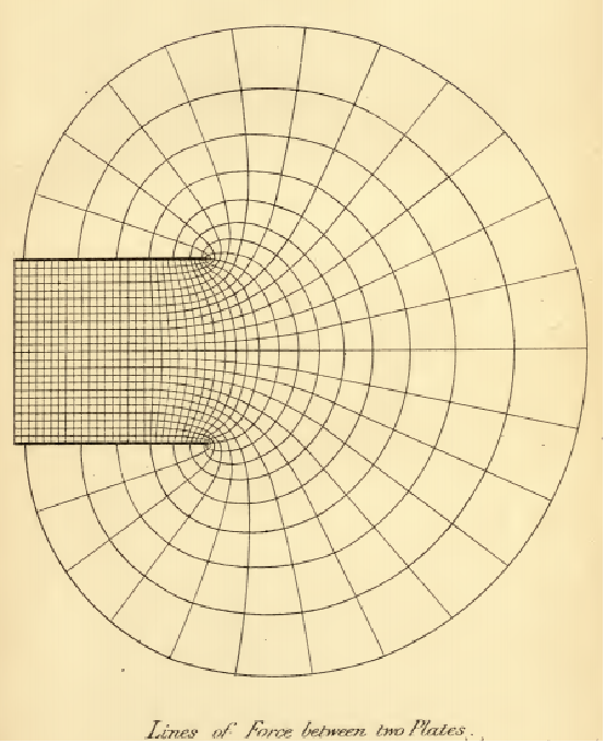
This requires different branches of the inverse of ![]() :
:
f[z_] := z + E^zInverseFunction[f][z]top = ComplexContourPlot[ReIm[z - ProductLog[1, E^z]], {z, -3π + π I, 2π + 3 π I}]Plot the middle part, taking care to match the contours in the upper part:
middle = ComplexContourPlot[ReIm[z - ProductLog[0, E^z]], {z, -3π - π I, 2π + π I}, Contours -> {Range[-10, 2, 0.25], Range[-3, 3, 0.5]}]bottom = ComplexContourPlot[ReIm[z - ProductLog[-1, E^z]], {z, -3π - 3π I, 2π - π I}]Show all three together to recreate Maxwell's image:
Show[top, middle, bottom,
	Graphics[{Thick, Red, Line[{{-3π, π}, {-1, π}}],
	Line[{{-3π, -π}, {-1, -π}}]}],
	PlotRange -> All]
Other Applications (2)
Show iterations of Newton's method:
f[z_] := z^5 - 2z^4 + 10z^3 - 2z^2 + 2z - 4{min, {steps}} = Reap[FindRoot[f[z], {z, 2 + I}, StepMonitor :> Sow[z]]];sg = ComplexListPlot[steps, PlotRange -> All, Joined -> True, PlotStyle -> White, Mesh -> All];Plot the contour lines for the function:
cg = ComplexContourPlot[Abs[f[z]], {z, -I, 2 + I}];Show[cg, sg]ComplexContourPlot[Evaluate@Table[Abs[z^2 - E^I θ] == 1, {θ, 0, 2π, (π/4)}], {z, 1.5}]Properties & Relations (9)
ComplexContourPlot is a special case of ContourPlot:
{ComplexContourPlot[Re[z^2], {z, -2 - 2I, 2 + 2I}],
	ContourPlot[Re[(x + I y)^2], {x, -2, 2}, {y, -2, 2}]}
ComplexContourPlot automatically suppresses shading for two or more functions:
{ComplexContourPlot[ReIm[z^2], {z, -2 - 2I, 2 + 2I}],
	ContourPlot[ReIm[(x + I y)^2], {x, -2, 2}, {y, -2, 2}, ContourShading -> None]}
ComplexRegionPlot plots regions over the complexes:
ComplexRegionPlot[Abs[Log[z]] < 1, {z, 3}]ComplexPlot shows the argument and magnitude of a function using color:
ComplexPlot[Log[z], {z, 3}]Use ComplexPlot3D to use the ![]() axis for the magnitude:
axis for the magnitude:
ComplexPlot3D[Log[z], {z, 3}]Use ComplexArrayPlot for arrays of complex numbers:
ComplexArrayPlot[Table[x ^ 3 + I y ^ 2, {x, -2, 2, 0.1}, {y, -2, 2, 0.1}]]Use ReImPlot and AbsArgPlot to plot complex values over the real numbers:
ReImPlot[Log[x], {x, -3, 3}]AbsArgPlot[Log[x], {x, -3, 3}]Use ComplexListPlot to show the location of complex numbers in the plane:
ComplexListPlot[RandomComplex[{-3 - 3I, 3 + 3I}, 100]]ComplexStreamPlot and ComplexVectorPlot treat complex numbers as directions:
ComplexStreamPlot[Log[z], {z, 3}]ComplexVectorPlot[Log[z], {z, 3}]Possible Issues (1)
Since Arg[f] cannot exceed ![]() , ComplexContourPlot will usually not render branch cuts:
, ComplexContourPlot will usually not render branch cuts:
ComplexContourPlot[Arg[Log[Gamma[z]]] == π, {z, -5 - 5I, 5 + 5I}]Text
Wolfram Research (2020), ComplexContourPlot, Wolfram Language function, https://reference.wolfram.com/language/ref/ComplexContourPlot.html.
CMS
Wolfram Language. 2020. "ComplexContourPlot." Wolfram Language & System Documentation Center. Wolfram Research. https://reference.wolfram.com/language/ref/ComplexContourPlot.html.
APA
Wolfram Language. (2020). ComplexContourPlot. Wolfram Language & System Documentation Center. Retrieved from https://reference.wolfram.com/language/ref/ComplexContourPlot.html