


DiscreteWaveletTransform
DiscreteWaveletTransform[data]
gives the discrete wavelet transform (DWT) of an array of data.
DiscreteWaveletTransform[data,wave]
gives the discrete wavelet transform using the wavelet wave.
DiscreteWaveletTransform[data,wave,r]
gives the discrete wavelet transform using r levels of refinement.
Details and Options

- DiscreteWaveletTransform gives a DiscreteWaveletData object representing a tree of wavelet coefficient arrays.
- Properties of the DiscreteWaveletData dwd can be found using dwd["prop"], and a list of available properties can be found using dwd["Properties"].
- The data can be any of the following:
-
list arbitrary-rank numerical array image arbitrary Image object audio an Audio or sampled Sound object - The resulting wavelet coefficients are arrays of the same depth as the input data.
- The possible wavelets wave include:
-
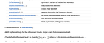
BattleLemarieWavelet[…] Battle–Lemarié wavelets based on B-spline BiorthogonalSplineWavelet[…] B-spline-based wavelet CoifletWavelet[…] symmetric variant of Daubechies wavelets DaubechiesWavelet[…] the Daubechies wavelets HaarWavelet[…] classic Haar wavelet MeyerWavelet[…] wavelet defined in the frequency domain ReverseBiorthogonalSplineWavelet[…] B-spline-based wavelet (reverse dual and primal) ShannonWavelet[…] sinc function-based wavelet SymletWavelet[…] least asymmetric orthogonal wavelet - The default wave is HaarWavelet[].
- With higher settings for the refinement level r, larger-scale features are resolved.
- The default refinement level r is given by
![TemplateBox[{{{InterpretationBox[{log, _, DocumentationBuild`Utils`Private`Parenth[2]}, Log2, AutoDelete -> True], (, n, )}, +, {1, /, 2}}}, Floor]](Files/DiscreteWaveletTransform.en/1.png "TemplateBox[{{{InterpretationBox[{log, _, DocumentationBuild`Utils`Private`Parenth[2]}, Log2, AutoDelete -> True], (, n, )}, +, {1, /, 2}}}, Floor]") , where
, where  is the minimum dimension of data. »
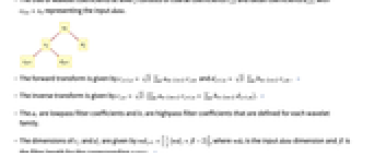
 - The tree of wavelet coefficients at level
 consists of coarse coefficients
  and detail coefficients
  , with
  representing the input data.
 - The forward transform is given by
 and
and  . »
. » - The inverse transform is given by
 . »
. » - The
 are lowpass filter coefficients and
  are highpass filter coefficients that are defined for each wavelet family.
 - The dimensions of
 and
and  are given by
 ![wd_(j+1)=TemplateBox[{{{1, /, 2}, , {(, {{wd, _, j}, +, fl, -, 2}, )}}}, Ceiling]](Files/DiscreteWaveletTransform.en/15.png "wd_(j+1)=TemplateBox[{{{1, /, 2}, , {(, {{wd, _, j}, +, fl, -, 2}, )}}}, Ceiling]") , where
, where  is the input data dimension and fl is the filter length for the corresponding wspec. »
 - The following options can be given:
-
Method Automatic method to use Padding "Periodic" how to extend data beyond boundaries WorkingPrecision MachinePrecision precision to use in internal computations - The settings for Padding are the same as those available in ArrayPad.
- InverseWaveletTransform gives the inverse transform.
Examples
open all close allBasic Examples (3)
Compute a discrete wavelet transform using the HaarWavelet:
Use Normal to view all coefficients:
Use dwd[…,"Audio"] to extract coefficient signals:
Compute the inverse transform:
Transform an Image object:
Scope (36)
Basic Uses (6)
The resulting DiscreteWaveletData represents a tree of transform coefficients:
The inverse transform reconstructs the input:
Useful properties can be extracted from the DiscreteWaveletData object:
Get a full list of properties:
Get data and coefficient dimensions:
Use Normal to get all wavelet coefficients explicitly:
Also use All as an argument to get all coefficients:
Use Automatic to get only the coefficients used in the inverse transform:
Use the "TreeView" or "WaveletIndex" to find out what wavelet coefficients are available:
Extract specific coefficient arrays:
Extract several wavelet coefficients corresponding to the list of wavelet index specifications:
Extract all coefficients whose wavelet indexes match a pattern:
The Automatic coefficients are used by default in functions like WaveletListPlot:
Use a higher refinement level to increase the frequency resolution:
With a smaller refinement level, more signal energy is left in {0,0,0}:
With further refinement, {0,0,0} is resolved into further components:
Wavelet Families (10)
Compute the discrete wavelet transform using different wavelet families:
Use different families of wavelets to capture different features:
HaarWavelet (default):
Vector Data (6)
Plot the coefficients over a common horizontal axis using WaveletListPlot:
Plot against a common vertical axis:
Visualize coefficients as a function of time and refinement level using WaveletScalogram:
The coefficient indexes appear as tooltips when the mouse pointer is moved over a coefficient:
All coefficients are small except coarse coefficients {0,0,…}:
Data oscillating at the highest resolvable frequency (Nyquist frequency):
Only the first detail coefficient {1} is not small:
Data with large discontinuities:
Coarse coefficients {0,…} have the same large-scale structure as the data:
Detail coefficients are sensitive to discontinuities:
Data with both spatial and frequency structure:
Coarse coefficients {0,…} track the local mean of the data:
The first detail coefficient identifies the oscillatory region:
Matrix Data (5)
Compute a two-dimensional discrete wavelet transform:
View the tree of wavelet coefficients:
Inverse transform to get back the original signal:
Use WaveletMatrixPlot to visualize the different wavelet coefficients:
WaveletMatrixPlot of wavelet transform at a higher refinement level:
In two dimensions, the vector of filtering operations in each direction can be computed:
Interpreting these vectors as binary digit expansions results in wavelet index numbers:
Get the lowpass and highpass filters for a Haar wavelet:
The resulting 2D filters are outer products of filters in the two directions:
Wavelet transform of step data:
Data with a vertical discontinuity:
Only the vertical detail coefficients, wavelet index {…,1}, are nonzero:
Data with horizontal discontinuity:
Only the horizontal detail coefficients, wavelet index {…,2}, are nonzero:
Data with diagonal discontinuity:
Only the diagonal detail coefficients, wavelet index {…,3}, are nonzero:
Array Data (2)
Compute a three-dimensional discrete wavelet transform:
Tree view of all coefficients:
Inverse transform to get back the original signal:
Wavelet transform of a three-dimensional cross array:
Visualize wavelet coefficients:
Energy of the original data is conserved within the transformed coefficients:
Image Data (4)
Transform an Image object:
The inverse transform yields a reconstructed Image object:
Wavelet coefficients are normally given as lists of data for each image channel:
Get all coefficients as Image objects instead:
Get raw Image objects with no rescaling of color levels:
Get the inverse transform of the {0,1} coefficient as an Image object:
Plot coefficients used in the inverse transform in a hierarchical grid using WaveletImagePlot:
Image wavelet coefficients lie outside the valid range of ImageType:
"ImageFunction"->Identity gives an unnormalized image wavelet coefficient:
The color channels lie outside its valid 0 to 1 range:
By default, "ImageFunction"->ImageAdjust is used to normalize coefficients:
Sound Data (3)
Transform a Sound object:
The inverse transform yields a reconstructed Sound object:
By default, coefficients are given as lists of data for each sound channel:
Get the {0,1} coefficient as a Sound object:
Inverse transform of {0,0,1} coefficient as a Sound object:
Browse all coefficients using a MenuView:
Generalizations & Extensions (3)
DiscreteWaveletTransform works on arrays of symbolic quantities:
Inverse transform recovers the input exactly:
Specify any internal working precision:
Options (5)
Padding (2)
WorkingPrecision (3)
By default, WorkingPrecision->MachinePrecision is used:
Use higher-precision computation:
With numbers close to zero, accuracy is the better indicator of the number of correct digits:
Use WorkingPrecision->∞ for exact computation:
Applications (11)
Wavelet Compression (1)
Compress data by finding a representation with few nonzero coefficients:
SymletWavelet[n] has n vanishing moments and represents polynomials of degree n:
Count counts the number of wavelet coefficients close to 0:
Detect Discontinuities and Edges (2)
Energy Comparison (1)
Denoising (3)
Perform energy-dependent thresholding:
Computing the fraction of energy contained at each refinement level:
Set wavelet coefficients containing less than 1% energy to zero:
Perform an amplitude-dependent thresholding:
Use WaveletThreshold to perform "Universal" thresholding:
Use Stein's unbiased risk estimator smoothing:
Denoise an Image:
Perform "Soft" thresholding with threshold value "SURE" computed adaptively at each level:
Frequency Filtering (1)
Wavelet transforms can be used to filter frequencies:
To filter out the two signals, first perform a wavelet transform:
Use WaveletListPlot to visualize frequency distribution:
To filter low frequencies, keep only the coarse coefficients:
To filter high frequencies, keep only the detail coefficients:
Finance (3)
Extract the stock price trend for IBM since January 1, 2000:
The trend of the series is captured in the lowpass filter coefficients:
Thresholding all detail coefficients and inverting the series gives the trend:
Detail coefficients captured the detrended series:
Remove the trend by removing the coarse coefficients and inverting:
Study variance of returns in a financial time series:
Perform a wavelet transform using HaarWavelet and SymletWavelet:
Since the GE return series does not exhibit low-frequency oscillations, higher-scale detail coefficients do not indicate large variations from zero:
Although both filters will capture the variance of the series, they distribute it differently because of their approximate bandpass properties:
SymletWavelet isolates features in a certain frequency interval better than HaarWavelet:
Properties & Relations (15)
DiscreteWaveletPacketTransform computes the full tree of wavelet coefficients:
DiscreteWaveletTransform computes a subset of the full tree of coefficients:
DiscreteWaveletTransform coefficients halve in length with each level of refinement:
Rotated data gives different coefficients:
StationaryWaveletTransform coefficients have the same length as the original data:
Rotated data gives rotated coefficients:
Multidimensional discrete wavelet transform is related to one-dimensional packet transform:
For Haar wavelet (default) and data length ![]() , the computed coefficients are identical:
, the computed coefficients are identical:
The default refinement is given by ![]() :
:
The energy norm is conserved for orthogonal wavelet families:
The energy norm is approximately conserved for biorthogonal wavelet families:
The mean of the data is captured at the maximum refinement level of the transform:
Extract the coefficient for the maximum refinement level:
Compensate for the ![]() normalization at each refinement level:
normalization at each refinement level:
The sum of inverse transforms from individual coefficient arrays gives the original data:
Individually inverse transform each wavelet coefficient array:
The sum gives the original data:
Compute discrete wavelet coefficients for periodic data:
Define filter coefficients to have compact support:
Coarse coefficients at level ![]() are given by
are given by ![]() , with
, with ![]() :
:
Detail coefficients at level ![]() are given by
are given by ![]() :
:
Compute a partial discrete inverse wavelet transform:
Define filter coefficients to have compact support:
Coarse coefficients at level ![]() are given:
are given:
Detail coefficients at level ![]() are given:
are given:
Inverse wavelet transform at level ![]() is given by
is given by ![]() :
:
Reconstruct coarse coefficients {0,0} at refinement level ![]() :
:
Reconstruct coarse coefficients {0} at refinement level ![]() :
:
Compute the dimensions of wavelet coefficients:
At refinement level ![]() , the dimensions of wavelet coefficients are given by
, the dimensions of wavelet coefficients are given by ![]() , where
, where ![]() represents dimensions of input data:
represents dimensions of input data:
Compare ![]() dimensions with coefficient dimensions in dwd:
dimensions with coefficient dimensions in dwd:
Compute a Haar discrete wavelet transform in one dimension:
Compute {0} and {1} wavelet coefficients:
Compare with DiscreteWaveletTransform:
In two dimensions, a separate filter is applied in each dimension:
Lowpass and highpass filters for Haar wavelet:
Haar wavelet transform of matrix data:
Compare with DiscreteWaveletTransform using HaarWavelet:
Image channels are transformed individually:
Combine {0} coefficients of separately transformed image channels:
Compare with {0} coefficient of DiscreteWaveletTransform of the original image:
DWT is similar to LiftingWaveletTransform with extra coefficients needed for padding:
Possible Issues (1)
Text
Wolfram Research (2010), DiscreteWaveletTransform, Wolfram Language function, https://reference.wolfram.com/language/ref/DiscreteWaveletTransform.html (updated 2017).
CMS
Wolfram Language. 2010. "DiscreteWaveletTransform." Wolfram Language & System Documentation Center. Wolfram Research. Last Modified 2017. https://reference.wolfram.com/language/ref/DiscreteWaveletTransform.html.
APA
Wolfram Language. (2010). DiscreteWaveletTransform. Wolfram Language & System Documentation Center. Retrieved from https://reference.wolfram.com/language/ref/DiscreteWaveletTransform.html