


LaplaceTransform
LaplaceTransform[f[t],t,s]
gives the symbolic Laplace transform of f[t] in the variable t as F[s] in the variable s.
LaplaceTransform[f[t],t,![]() ]
]
gives the numeric Laplace transform at the numerical value ![]() .
.
LaplaceTransform[f[t1,…,tn],{t1,…,tn},{s1,…,sn}]
gives the multidimensional Laplace transform of f[t1,…,tn].
Details and Options
- Laplace transforms are typically used to transform differential and partial differential equations to algebraic equations, solve and then inverse transform back to a solution.
- Laplace transforms are also extensively used in control theory and signal processing as a way to represent and manipulate linear systems in the form of transfer functions and transfer matrices. The Laplace transform and its inverse are then a way to transform between the time domain and frequency domain.
- The Laplace transform of a function
 is defined to be
  .
. - The multidimensional Laplace transform is given by
 .
. - The integral is computed using numerical methods if the third argument, s, is given a numerical value.
- The asymptotic Laplace transform can be computed using Asymptotic.
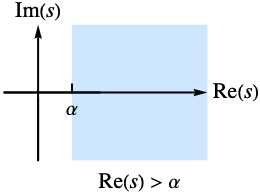
- The Laplace transform of
 exists only for complex values of s in a half-plane
  .
. - The lower limit of the integral is effectively taken to be
 , so that the Laplace transform of the Dirac delta function
  is equal to 1. »
 - The following options can be given:
-
AccuracyGoal Automatic digits of absolute accuracy sought Assumptions $Assumptions assumptions to make about parameters GenerateConditions False whether to generate answers that involve conditions on parameters Method Automatic method to use PerformanceGoal $PerformanceGoal aspects of performance to optimize PrecisionGoal Automatic digits of precision sought PrincipalValue False whether to find Cauchy principal value WorkingPrecision Automatic the precision used in internal computations - Use GenerateConditions"ConvergenceRegion" to obtain the region of convergence for the Laplace transform.
- In TraditionalForm, LaplaceTransform is output using
 . »
. »
Examples
open all close allBasic Examples (4)
Compute the Laplace transform of a function:
LaplaceTransform[ Exp[-t], t, s]f[t_] := t UnitStep[t - 1]Plot[f[t], {t, 0, 3}]Compute its Laplace transform:
LaplaceTransform[f[t], t, s]Compute the transform at a single point:
LaplaceTransform[f[t], t, 0.3]Compute the Laplace transform of a multivariate function:
LaplaceTransform[x Exp[-y], {x, y}, {p, q}]Define a multivariate piecewise function:
f[x_, y_] = UnitStep[x + y - 1] x;Plot3D[f[x, y], {x, 0, 1}, {y, 0, 1}]Compute its Laplace transform:
LaplaceTransform[f[x, y], {x, y}, {p, q}]//FullSimplifyScope (67)
Basic Uses (4)
Laplace transform of a function for a symbolic parameter s:
LaplaceTransform[1, t, s]Laplace transforms of trigonometric functions:
LaplaceTransform[Sin[ω t], t, s]LaplaceTransform[Cos[ω t], t, s]Evaluate the Laplace transform for a numerical value of the parameter s:
LaplaceTransform[Sin[t], t, 1.2]TraditionalForm formatting:
LaplaceTransform[f[x], x, s]//TraditionalFormElementary Functions (13)
Laplace transform of a power function:
LaplaceTransform[t^n, t, s]LaplaceTransform[Sqrt[t], t, s]Laplace transforms of polynomials:
LaplaceTransform[3t ^ 2 + 5t - 7, t, s]LaplaceTransform[Sum[a[i]t^i, {i, 1, n}], t, s]LaplaceTransform[E ^ (-a t), t, s]Product of an exponential and a linear function:
LaplaceTransform[(1 + a t)Exp[a t], t, s]//TogetherExpressions involving trigonometric functions:
LaplaceTransform[Exp[a t] Sin[ω t], t, s]LaplaceTransform[(1/2ω)(Sin[ω t] + ω t Cos[ω t]), t, s]//SimplifyExpressions involving hyperbolic functions:
LaplaceTransform[(b Sinh[a t] - a Sinh[b t]/a^2 - b^2), t, s]//SimplifyLaplaceTransform[t Cosh[a t], t, s]Ratio of an exponential and a linear function:
LaplaceTransform[(Exp[t] - 1/t), t, s]Ratio of sine and linear functions:
LaplaceTransform[(Sin[3 t]/t), t, s]Composition of elementary functions:
LaplaceTransform[(a Exp[-(a^2/4 t)]/2 Sqrt[π] t^3 / 2), t, s, Assumptions -> a > 0]LaplaceTransform[Sin[t ^ 2], t, s]LaplaceTransform[Log[t], t, s]Product of logarithmic and power functions:
LaplaceTransform[t^ν - 1Log[t], t, s]Square of a logarithmic function:
LaplaceTransform[Log[t] ^ 2, t, s]Special Functions (10)
Laplace transform of error and square root functions composition:
Simplify[LaplaceTransform[(1/Sqrt[a])Erf[Sqrt[a t]], t, s], Assumptions -> {a > 0, s > 0}]LaplaceTransform[BesselJ[0, a t], t, s]LaplaceTransform[BesselI[0, a t], t, s]Products involving Bessel functions:
Simplify[LaplaceTransform[((t/2a))^ν - 1 / 2BesselJ[ν - 1 / 2, a t], t, s], Assumptions -> a > 0]Simplify[LaplaceTransform[((t/2a))^ν - 1 / 2BesselI[ν - 1 / 2, a t], t, s], Assumptions -> a > 0]LaplaceTransform[SinIntegral[t], t, s]LaplaceTransform[LaguerreL[n, t], t, s]LaplaceTransform[AiryAi[t], t, s]LaplaceTransform[((1 + t)^n/Sqrt[t])ChebyshevT[n, (1 - t/1 + t)], t, s]LaplaceTransform[(StruveH[1 / 2, a t]/Sqrt[t]), t, s]LaplaceTransform[FresnelC[Sqrt[(2/Pi)]Sqrt[a * t]], t, s]LaplaceTransform[Gamma[nu, a / t], t, s]LaplaceTransform[t^5 / 3HypergeometricPFQ[{-(7/4), (11/4)}, {1, (8/3)}, t], t, s]Piecewise Functions (9)
Laplace transform of a piecewise function:
f[t_] = Piecewise[{{t, 0 ≤ t ≤ 1}, {1, t > 1}}];Plot[f[t], {t, 0, 3}]LaplaceTransform[f[t], t, s]Restriction of a sine function to a half-period:
f[t_] = Piecewise[{{Sin[ω t], 0 < t < (π/ω)}, {0, (π/ω) ≤ t}}];Plot[f[t] /. ω -> π, {t, 0, 2}]LaplaceTransform[f[t], t, s, Assumptions -> ω > 0]Exponential function with a left cutoff:
f[t_] = Piecewise[{{2, t ≤ 1}, {Exp[t], t > 1}}];Plot[f[t], {t, 0, 2}]LaplaceTransform[f[t], t, s]//FullSimplifyf[t_] = Piecewise[{{t, 0 ≤ t ≤ 1}, {2 - t, 1 < t ≤ 2}, {0, 2 < t }}];Plot[f[t], {t, 0, 4}]LaplaceTransform[f[t], t, s]Polynomial function with a left cutoff:
f[t_] = Piecewise[{{0, 0 ≤ t < 1}, {(t - 1)^2, 1 ≤ t}}];Plot[f[t], {t, 0, 3}]LaplaceTransform[f[t], t, s]LaplaceTransform[Ramp[t - a], t, s, Assumptions -> a > 0]LaplaceTransform[UnitStep[t - a], t, s, Assumptions -> a > 0]Product of UnitStep and cosine functions:
LaplaceTransform[UnitStep[t - π]Cos[t - π], t, s]Laplace transform of Floor:
LaplaceTransform[Floor[t], t, s]Plot[Floor[t], {t, 0, 10}]Periodic Functions (5)
Laplace transform of SquareWave:
LaplaceTransform[SquareWave[t], t, s]Plot[SquareWave[t], {t, 0, 4}]LaplaceTransform[TriangleWave[t], t, s]Plot[TriangleWave[t], {t, 0, 4}]LaplaceTransform[SawtoothWave[t], t, s]Plot[SawtoothWave[t], {t, 0, 6}]Full-wave-rectified function with period ![]() :
:
LaplaceTransform[RealAbs[Sin[t]], t, s]//FullSimplifyPlot[RealAbs[Sin[t]], {t, 0, 12}]f[t_] = Piecewise[{{Sin[t], 0 ≤ Mod[(t/π), 2] ≤ 1}, {0, 1 < Mod[(t/π), 2] < 2}}];LaplaceTransform[f[t], t, s]Plot[f[t], {t, 0, 24}]Generalized Functions (5)
Laplace transform of HeavisideTheta:
LaplaceTransform[HeavisideTheta[t], t, s]LaplaceTransform[DiracDelta[t - 1], t, s]Derivative of DiracDelta:
LaplaceTransform[DiracDelta'[t - 1], t, s]Plot[HeavisideLambda[t - 1], {t, 0, 4}]LaplaceTransform[HeavisideLambda[t - 1], t, s]LaplaceTransform[HeavisidePi[t - (3/2)], t, s]Plot[HeavisidePi[t - (3/2)], {t, 0, 3}]Multivariate Functions (9)
Bivariate Laplace transform of a constant:
LaplaceTransform[1, {x, y}, {p, q}]LaplaceTransform[Exp[a x + b y], {x, y}, {p, q}]LaplaceTransform[(x^m y^n/Gamma[m + 1]Gamma[n + 1]), {x, y}, {p, q}]LaplaceTransform[BesselJ[0, 2 Sqrt[a x y]], {x, y}, {p, q}]//SimplifyLaplaceTransform[(1/Sqrt[π (x + y)]), {x, y}, {p, q}, Assumptions -> {p > 0, q > 0}]Composition of cosine and square root:
LaplaceTransform[(Cos[Sqrt[x y ]]/Sqrt[x y ]), {x, y}, {p, q}]Laplace transform of a multivariate power function:
LaplaceTransform[(x^m y^nz^k/Gamma[m + 1]Gamma[n + 1]Gamma[k + 1]), {x, y, z}, {p, q, r}]LaplaceTransform[Cos[x + y + z], {x, y, z}, {p, q, r}]//SimplifyAssuming[{p > 0, q > 0, r > 0}, FullSimplify[LaplaceTransform[Log[x y z], {x, y, z}, {p, q, r}]]]Formal Properties (6)
The Laplace transform is a linear operator:
LaplaceTransform[a f[t] + b g[t], t, s]Laplace transform of ![]() is the Laplace transform of
is the Laplace transform of ![]() evaluated at
evaluated at ![]() :
:
LaplaceTransform[Exp[a t]f[t], t, s]Laplace transform of a first-order derivative:
LaplaceTransform[f'[t], t, s]Laplace transform of a second-order derivative:
LaplaceTransform[f''[t], t, s]Laplace transform of a product with monomials:
LaplaceTransform[t f[t], t, s]LaplaceTransform[t ^ 2 f[t], t, s]Laplace transform threads itself over equations:
LaplaceTransform[f'[t] == Log[t], t, s]Numerical Evaluation (3)
Calculate the Laplace transform at a single point:
LaplaceTransform[(Erf[t]/Sqrt[t]), t, 14.2]Alternatively, calculate the Laplace transform symbolically:
LaplaceTransform[(Erf[t]/Sqrt[t]), t, s]Then evaluate it for specific value of ![]() :
:
N[% /. s -> Rationalize[14.2], 20]Plot the Laplace transform using numerical values only:
f[s_ ? NumericQ] := LaplaceTransform[(Erf[t]/Sqrt[t]), t, s]Plot[f[s], {s, 0, 5}]For some functions, the Laplace transform cannot be evaluated symbolically:
LaplaceTransform[(Erfc[t]/t^2 + 1), t, s]Evaluate the Laplace transform numerically and plot it:
f[s_ ? NumericQ] := LaplaceTransform[(Erfc[t]/t^2 + 1), t, s]f[0.4]Plot[f[s], {s, 0, 10}]Calculate a multivariate Laplace transform at a single point in the plane:
LaplaceTransform[(1/x + y + 1), {x, y}, {5.4, 4.5}]Fractional Calculus (3)
Laplace transform of the MittagLefflerE functions:
LaplaceTransform[(-MittagLefflerE[(1/2), (1/2), (Sqrt[t]/2)] + MittagLefflerE[(1/2), (1/2), (2 Sqrt[t]/3)]/Sqrt[t]), t, s]ComplexPlot in the ![]() -domain:
-domain:
ComplexPlot[%, {s, -1 - I, 1 + I}]Inverse Laplace transform to the time domain:
InverseLaplaceTransform[-(2/-1 + 2 Sqrt[s]) + (3/-2 + 3 Sqrt[s]), s, t]Laplace transform of the MittagLefflerE functions involving parameters:
LaplaceTransform[MittagLefflerE[α, a t^α], t, s]Inverse Laplace transform to the time domain:
InverseLaplaceTransform[%, s, t, Assumptions -> α > 0]Laplace transform of the CaputoD fractional derivative:
LaplaceTransform[CaputoD[f[t], {t, 3 / 2}], t, s]% /. {f[t_] -> Sin[t], f'[t_] -> Cos[t]}//SimplifyCompare this with the LaplaceTransform of the CaputoD derivative of the sine function:
CaputoD[Sin[t], {t, 3 / 2}]LaplaceTransform[%, t, s]//FullSimplifyOptions (4)
Assumptions (1)
Specify the range for a parameter using Assumptions:
LaplaceTransform[ArcTan[t / a], t, s, Assumptions -> a > 0]GenerateConditions (1)
Use GenerateConditions->True to get parameter conditions for when a result is valid:
LaplaceTransform[E ^ (-a t ^ 2), t, s, GenerateConditions -> True]Principal Value (1)
The Laplace transform of the following function is not defined due to the singularity at ![]() :
:
LaplaceTransform[(Sin[t]/t - 1), t, s]Use PrincipalValue to obtain the Cauchy principal value for the integral:
LaplaceTransform[(Sin[t]/t - 1), t, s, PrincipalValue -> True]//FullSimplifyWorking Precision (1)
Use WorkingPrecision to obtain a result with arbitrary precision:
LaplaceTransform[(Exp[-t^2]/t^2 + 5t + 2), t, 15.7]LaplaceTransform[(Exp[-t^2]/t^2 + 5t + 2), t, 15.7, WorkingPrecision -> 10]LaplaceTransform[(Exp[-t^2]/t^2 + 5t + 2), t, 15.7, WorkingPrecision -> 20]Applications (12)
Ordinary Differential Equations (5)
Solve a differential equation using Laplace transforms:
LaplaceTransform[y''[t] + y[t] == 1, t, s] /. {y[0] -> 0, y'[0] -> 0}Solve for the Laplace transform:
Solve[%, LaplaceTransform[y[t], t, s]]InverseLaplaceTransform[%, s, t]Plot[y[t] /. %, {t, 0, 5Pi}]Find the solution directly using DSolve:
DSolve[{y''[t] + y[t] == 1, y[0] == 0, y'[0] == 0}, y[t], t]Solve the following differential equation:
eqn = 4y''[t] - y[t] == UnitStep[t - 1];Solve for the Laplace transform:
Solve[LaplaceTransform[eqn, t, s] /. {y[0] -> 0, y'[0] -> 1 / 25}, LaplaceTransform[y[t], t, s]]InverseLaplaceTransform[%, s, t]//FullSimplifyPlot[y[t] /. %, {t, 0, 3}]Solve an RL circuit to find the current ![]() :
:
Solve[LaplaceTransform[L i'[t] + R i[t] == E0 Sin[ω t], t, s] /. i[0] -> 0, LaplaceTransform[i[t], t, s]]InverseLaplaceTransform[%, s, t]//ExpandVerify with DSolveValue:
DSolveValue[{L i'[t] + R i[t] == E0 Sin[ω t], i[0] == 0}, i[t], t]//ExpandGreen's function for an RL circuit:
Solve[LaplaceTransform[L i'[t] + R i[t] == DiracDelta[t - τ], t, s] /. i[0] -> 0, LaplaceTransform[i[t], t, s]]GreenF[t_, τ_] = i[t] /. Assuming[τ > 0, Refine[InverseLaplaceTransform[%, s, t]]][[1]]Use the Green's function to solve the RL circuit:
Integrate[GreenF[t, τ] * E0 Sin[ω τ], {τ, 0, ∞}, Assumptions -> {t > 0, R > 0, L > 0}]//ExpandSolve[LaplaceTransform[{y'[t] == -z[t], z'[t] == y[t]}, t, s] /. {y[0] -> 1, z[0] -> 0}, LaplaceTransform[{y[t], z[t]}, t, s]]InverseLaplaceTransform[%, s, t]Fractional Differential Equations (3)
Solve a fractional-order differential equation using Laplace transforms:
LaplaceTransform[CaputoD[y[t], {t, 5 / 3}] + y[t] == 1, t, s] /. {y[0] -> 0, y'[0] -> -1}Solve for the Laplace transform:
Solve[%, LaplaceTransform[y[t], t, s]]InverseLaplaceTransform[%, s, t]Plot[y[t] /. %, {t, 0, 6}]Find the solution directly using DSolve:
DSolve[{CaputoD[y[t], {t, 5 / 3}] + y[t] == 1, y[0] == 0, y'[0] == -1}, y[t], t]Solve the following fractional integro-differential equation:
eqn = CaputoD[y[t], {t, 1 / 2}] - CaputoD[y[t], {t, -1 / 2}] == 1;Solve for the Laplace transform:
Solve[LaplaceTransform[eqn, t, s] /. y[0] -> 0, LaplaceTransform[y[t], t, s]]InverseLaplaceTransform[%, s, t]Find the solution directly using DSolve:
DSolve[{eqn, y[0] == 0}, y[t], t]The following equation describes a fractional harmonic oscillator of order 1.9:
eqn = CaputoD[x[t], {t, 1.9}] + 5x[t] == 0;Solve for the Laplace transform:
Solve[LaplaceTransform[eqn, t, s] /. {x[0] -> 0, x'[0] -> 1}, LaplaceTransform[x[t], t, s]]InverseLaplaceTransform[%, s, t]Plot[x[t] /. %, {t, 0, 10}]Find the solution directly using DSolve:
DSolve[{eqn, x[0] == 0, x'[0] == 1}, x[t], t]Evaluation of Integrals (2)
Calculate the following integral:
Inactivate[Integrate[(u Sin[t u]/1 + u^2), {u, 0, ∞}], Integrate]Compute the Laplace transform and interchange the order of Laplace transform and integration:
Inactivate[Integrate[LaplaceTransform[(u Sin[t u]/1 + u^2), t, s], {u, 0, ∞}], Integrate]Perform the integration over ![]() :
:
Assuming[s > 0, Activate[%]]Use InverseLaplaceTransform to obtain the original integral:
InverseLaplaceTransform[%, s, t]Integrate[(u Sin[t u]/1 + u^2), {u, 0, ∞}, Assumptions -> t > 0]Integral involving the Bessel function:
Inactivate[Integrate[(BesselJ[k, u]/u^k - n + 1), {u, 0, ∞}], Integrate]Perform a change of variables ![]() and introduce an auxiliary variable
and introduce an auxiliary variable ![]() :
:
f[t_] = Inactivate[(1/2^k - n + 1)Integrate[v^(n/2) - 1((t/v))^(k/2)BesselJ[k, 2 Sqrt[v t]], {v, 0, ∞}], Integrate]Apply the Laplace transform and interchange the order of Laplace transform and integration:
Inactivate[(1/2^k - n + 1)Integrate[v^(n/2) - 1LaplaceTransform[((t/v))^(k/2)BesselJ[k, 2 Sqrt[v t]], t, s], {v, 0, ∞}], Integrate]Perform the integration over ![]() :
:
Assuming[{s > 0, n > 0}, Activate[%]]Use InverseLaplaceTransform to obtain ![]() :
:
f[t_] = InverseLaplaceTransform[%, s, t]The original integral equals ![]() :
:
f[t] /. t -> 1Integrate[(BesselJ[k, u]/u^k - n + 1), {u, 0, ∞} , GenerateConditions -> False]Other Applications (2)
Compute a Laplace transform using a series expansion:
f[t_] = Exp[-t^2];coeff = SeriesCoefficient[f[t], {t, 0, n}]The transformed series can be summed using Regularization:
Assuming[s > 0, Sum[LaplaceTransform[(coeff /. n -> 2n )t^2n, t, s], {n, 0, ∞}, Regularization -> "Borel"]]Verify the result directly using LaplaceTransform:
LaplaceTransform[Exp[-t^2], t, s]Laplace transform of Sinc using series expansions:
f[t_] = Sinc[t];Plot[f[t], {t, 0, 30}, PlotRange -> All]coeff = SeriesCoefficient[f[t], {t, 0, n}]Assuming[s > 0, Sum[LaplaceTransform[(coeff /. n -> 2n ) t^2n, t, s], {n, 0, ∞}]]LaplaceTransform[(Sin[t]/t), t, s]Properties & Relations (3)
Use Asymptotic to compute an asymptotic approximation:
Asymptotic[Inactive[LaplaceTransform][1 / (E ^ (t ^ 2) + t ^ 17), t, s], s -> Infinity]LaplaceTransform and InverseLaplaceTransform are mutual inverses:
InverseLaplaceTransform[LaplaceTransform[f[t], t, s], s, t]LaplaceTransform[InverseLaplaceTransform[g[s], s, t], t, s]LaplaceTransform[E ^ (-t ^ 2), t, s]InverseLaplaceTransform[%, s, t]Use NIntegrate for numerical approximation:
LaplaceTransform[1 / (1 + t ^ 2), t, s]% /. {s -> 0.4}NIntegrate computes the transform for numeric values of the Laplace parameter s:
NIntegrate[Exp[-0.4 t] / (1 + t ^ 2), {t, 0, Infinity}]Possible Issues (1)
Neat Examples (2)
LaplaceTransform done in terms of MeijerG:
LaplaceTransform[1 / (1 + t ^ 8), t, s]Create a table of basic Laplace transforms:
flist = {t^n, E ^ (a t), Sin[a t], t Sin[a t], Sinh[a t], DiracDelta[t - a],
Log[t], Floor[t], (1/Sqrt[a])Erf[Sqrt[a t]], BesselJ[n, t], BesselI[n, t], (2/Sqrt[π])Exp[-t^2]};Grid[Prepend[{#, Assuming[{a > 0, s > 0}, Simplify[LaplaceTransform[#1, t, s]]]}& /@ flist, {f[t], LaplaceTransform[f[t], t, s]}], IconizedObject[«Grid options»]]//TraditionalFormRelated Links
Text
Wolfram Research (1999), LaplaceTransform, Wolfram Language function, https://reference.wolfram.com/language/ref/LaplaceTransform.html (updated 2023).
CMS
Wolfram Language. 1999. "LaplaceTransform." Wolfram Language & System Documentation Center. Wolfram Research. Last Modified 2023. https://reference.wolfram.com/language/ref/LaplaceTransform.html.
APA
Wolfram Language. (1999). LaplaceTransform. Wolfram Language & System Documentation Center. Retrieved from https://reference.wolfram.com/language/ref/LaplaceTransform.html