



LogLinearPlot
LogLinearPlot[f,{x,xmin,xmax}]
生成一个函数 f 的对数-线性图,其自变量 x 取值范围为从 xmin 到 xmax.
LogLinearPlot[{f1,f2,…},{x,xmin,xmax}]
绘制几个函数 fi.
LogLinearPlot[{…,w[fi],…},…]
绘制特性由符号化封装 w 定义的 fi.
LogLinearPlot[…,{x}∈reg]
将变量 x 视为在几何区域 reg 中.
更多信息和选项
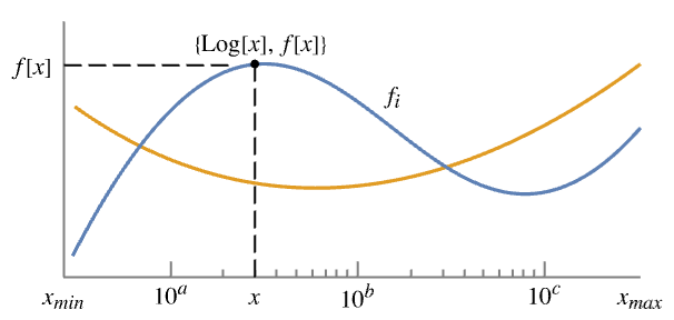
- LogLinearPlot 也被称为半对数图,因为该图有一个对数坐标轴和一个线性坐标轴.
- LogLinearPlot 使得对数函数以直线的方式呈现. 绘图可以涵盖非常大的定义域.
- LogLinearPlot 实际上生成一条 f 相对于 Log[x] 绘制的曲线,只是刻度表示 x 的原始值. 该函数可视化集合
 .
- 在 fi 运算结果不是实数或 Quantity 的 x 处会留下间隙.
- 范围限制 xmin 和 xmax 可以是实数或 Quantity 表达式.
- 区域 reg 可以是任意一维中的 RegionQ 对象.
- LogLinearPlot 将变量 x 视为本地变量,实际上相当于使用 Block.
- LogLinearPlot 有 HoldAll 属性,只在将特定值赋给 x 后才对 f 进行计算.
- 有些情况下,在将具体数值赋给 x 之前,用 Evaluate 以符号方式计算 f 可能更高效.
- 可将下列封装 w 用于 fi:
-
Annotation[fi,label] 为 fi 提供注释 Button[fi,action] 当 fi 的曲线被点中时执行 action Callout[fi,label] 用 callout 标注函数 Callout[fi,label,pos] 在相对位置 pos 处放置 callout EventHandler[fi,events] 为 fi 定义通用事件处理程序 Highlighted[fi,effect] 用某种效果动态突出显示 fi Highlighted[fi,Placed[effect,pos]] 在位置 pos 处用某种效果静态突出显示 fi Hyperlink[fi,uri] 将函数变成超链接 Labeled[fi,label] 标记函数 Labeled[fi,label,pos] 在相对位置 pos 处放置标签 Legended[fi,label] 在图例中标识函数 PopupWindow[fi,cont] 为函数添加弹出窗口 StatusArea[fi,label] 鼠标悬停时在状态栏中显示 Style[fi,styles] 用指定样式显示函数 Tooltip[fi,label] 为函数添加提示条 Tooltip[fi] 将函数作为提示条 - 可在多个层级上应用封装 w:
-
w[fi] 封装 fi w[{f1,…}] 封装 fi 的集合 w1[w2[…]] 使用嵌套封装 - 在 Callout、Labeled 和 Placed 中可使用以下位置 pos:
-
Automatic 自动放置标签 Above, Below, Before, After 在曲线周围的位置 x 在位置 x 处的曲线的附近 Scaled[s] 沿曲线的缩放位置 s {s,Above},{s,Below},… 沿曲线的在位置 s 处的相对位置 {pos,epos} 在曲线的相对位置 pos 处放置的标签中的 epos - LogLinearPlot 有和 Graphics 相同的选项,不同之处和更多选项如下所示: [所有选项的列表]
-
AspectRatio 1/GoldenRatio 高宽比 Axes True 是否画出坐标轴 ClippingStyle None 曲线被剪除处如何绘制 ColorFunction Automatic 如何确定曲线的颜色 ColorFunctionScaling True 是否缩放传递给 ColorFunction 的参数 EvaluationMonitor None 每次函数运算时要计算的表达式 Exclusions Automatic 不要包括的点 x ExclusionsStyle None 在被排除的点处绘制什么 Filling None 在每个曲线下加上的填充 FillingStyle Automatic 填充使用的样式 LabelingSize Automatic callout 和标签的最大尺寸 MaxRecursion Automatic 允许的递归细分的最大数量 Mesh None 在各曲线上绘制多少网格点 MeshFunctions {#1&} 如何确定网格点的放置 MeshShading None 怎样处理网格点之间区域的色调 MeshStyle Automatic 网格点的样式 Method Automatic 细化曲线的方法 PerformanceGoal $PerformanceGoal 优化的目标 PlotHighlighting Automatic 曲线的突出显示效果 PlotInteractivity $PlotInteractivity 是否允许交互元素 PlotLabel None 绘图的整体标签 PlotLabels None 用于曲线的标签 PlotLegends None 曲线的图例 PlotPoints Automatic 样本点的初始数目 PlotRange {Full,Automatic} 要包含的 y 的范围或其他值 PlotRangeClipping True 在绘图范围边界处是否进行剪切 PlotStyle Automatic 指定各个曲线的样式的图形指令 PlotTheme $PlotTheme 绘图的整体主题 RegionFunction (True&) 如何判定一个点是否应被包含 TargetUnits Automatic 要在图中显示的单位 WorkingPrecision MachinePrecision 内部计算中使用的精度 - ClippingStyle 的可能设置有:
-

Automatic 在剪除部分使用虚线 
None 省略曲线被剪除的部分 
style 在被剪除部分使用 style - 在多个绘图面板中显示单个曲线的 PlotLayout 的可能设置包括:
-
"Column" 在一列面板中使用不同曲线 "Row" 在一行面板中使用不同曲线 {"Column",k},{"Row",k} 使用 k 列或行 {"Column",UpTo[k]},{"Row",UpTo[k]} 使用至多 k 列或行 - 通过默认设置 Exclusions->Automatic 和 ExclusionsStyle->None,LogLinearPlot 在检测到的断点和奇点处断开曲线. Exclusions->None 则将断点和奇点连起来.
- Exclusions->{x1,x2,…} 等价于 Exclusions->{x==x1,x==x2,…}.
- PlotLegends 的典型设置包括:
-
None 没有图例 Automatic 自动确定图例 "Expressions" 用 f1, f2, … 作为图例的标签 {lbl1,lbl2,…} 用 lbl1, lbl2, … 作为图例的标签 Placed[lspec,…] 指定图例的放置 - PlotStylesty 指定每条曲线使用的样式. 可能的设置包括:
-
{sty1,sty2,…} 针对各个数据集的一系列样式 <"key"val,…> 针对不同层级的数据的样式元素 - 接受的键有:
-
"Base" 所有 fi 的整体样式 "Functions" 针对每个 fi 的样式列表 styi - ColorData["DefaultPlotColors"] 给出 PlotStyle 使用的默认颜色序列.
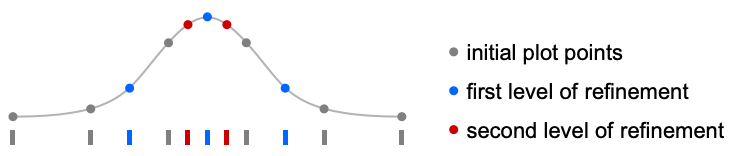
- LogLinearPlot 在 PlotPoints 指定的一些等距采样点对 f 进行初始求值. 然后使用自适应算法选择额外的采样点,将给定区间进行最多 MaxRecursion 次细分.
- 由于只使用了有限数的采样点,LogLinearPlot 可能会漏掉 f 的某些特性. 增大 PlotPoints 和 MaxRecursion 的设置通常可以补上这样的特性.
- 影响曲线的主题包括:
-

"ThinLines" 细的绘图线 
"MediumLines" 中等绘图线 
"ThickLines" 粗的绘图线 - MeshFunctions 和 RegionFunction 中函数的自变量是 x 和 y. ColorFunction 中的函数默认情况下使用这些自变量缩放后的形式.
- Highlighted 和 PlotHighlighting 可用的突出显示效果包括:
-
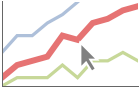
style 突出显示指定的曲线 
"Ball" 突出显示并标注曲线上指定的点 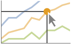
"Dropline" 突出显示并标注曲线上指定的点,同时绘制到坐标轴的准线 
"XSlice" 突出显示并标注垂直切片上的所有点 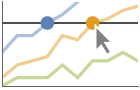
"YSlice" 突出显示并标注水平切片上的所有点 
Placed[effect,pos] 静态突出显示给定位置 pos - 突出显示的位置指定 pos 包括:
-
x, {x} 在 {x,y} 处突出显示,自动选择 y {x,y} 在 {x,y} 处突出显示 {pos1,pos2,…} 多个位置 posi - ScalingFunctions 的可能设置包括:
-
sy 缩放 y 轴 {sx,sy} 缩放 x 和 y 轴 - 常见的内置缩放函数 s 包括:
-
"Log" 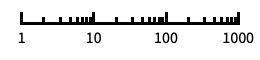
对数刻度,自动进行标记 "Log10" 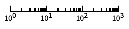
以 10 为底的对数刻度,用 10 的幂进行标记 "SignedLog" 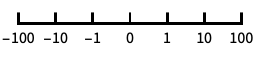
类似对数的刻度,包含 0 和负数 "Reverse" 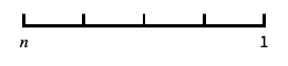
反转坐标的方向 "Infinite" 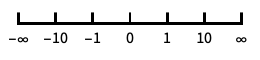
无穷刻度 - 如果为 x 方向指定了缩放函数,则在正常对数缩放之后应用.
所有选项的列表
范例
打开所有单元 关闭所有单元基本范例 (4)
LogLinearPlot[Tanh[x], {x, 1, 100}]LogLinearPlot[{Tanh[x], Erf[x]}, {x, 1, 100}, PlotLegends -> "Expressions"]LogLinearPlot[{Erf[x], Erfc[x]}, {x, 0.01, 10}, PlotLabels -> "Expressions"]LogLinearPlot[Erf[x], {x, 1, 100}, Filling -> Bottom]范围 (30)
采样 (7)
LogLinearPlot[Cos[x], {x, 0.1, 10}, Mesh -> All]LogLinearPlot[Abs[1 / (x - 5)], {x, 1, 10}]LogLinearPlot[Sqrt[(x - 3)(x - 5)], {x, 1, 10}]LogLinearPlot[Floor[Sqrt[x]], {x, 1, 100}]使用 PlotPoints 和 MaxRecursion 来控制自适应采样:
Grid@Table[LogLinearPlot[Sin[x], {x, 0.1, 10}, PlotPoints -> pp, MaxRecursion -> mr], {mr, {0, 1, 2}}, {pp, {5, 20}}]使用 PlotRange 探索感兴趣的区域:
{LogLinearPlot[{Erf[x] - Tanh[x]}, {x, 0.001, 100}], LogLinearPlot[{Erf[x] - Tanh[x]}, {x, 0.001, 100}, PlotRange -> {0, 1}]}使用 Exclusions 删除点或分裂生成的曲线:
LogLinearPlot[Tan[x], {x, 1, 15}, Exclusions -> {Cos[x] == 0}]添加标签和图例 (11)
用 Labeled 标记曲线:
LogLinearPlot[Evaluate@Table[Labeled[Log[n x] ^ 2, Log[n x] ^ 2], {n, 1, 3}], {x, 0.1, 3}]Table[LogLinearPlot[Labeled[x ^ Sin[x], "label", p], {x, 1, 6}, PlotLabel -> p], {p, {Above, Below, Before, After}}]用 PlotLabels 标记曲线:
LogLinearPlot[{Log[x], 1 / x}, {x, 1, 10}, PlotLabels -> {Log[x], 1 / x}]
LogLinearPlot[Labeled[Sin[x / Log[x]], "label", Log[5]], {x, 2, 100}]LogLinearPlot[Labeled[x ^ Sin[x], x ^ Sin[x], Scaled[0.3]], {x, 1, 2π}]LogLinearPlot[Labeled[x ^ Sin[x], x ^ Sin[x], {Scaled[0.3], Above}], {x, 1, 2π}]用 Callout 自动标记曲线:
LogLinearPlot[{Callout[Erf[x], Erf[x]], Callout[Erfc[x], Erfc[x]]}, {x, 0.01, 10}]LogLinearPlot[{Callout[Erf[x], Erf[x], 5], Callout[Erfc[x], Erfc[x], 0.05]}, {x, 0.01, 10}]LogLinearPlot[{x ^ Sin[x], x ^ Cos[x]}, {x, 1, 2π}, PlotLegends -> {x ^ Sin[x], x ^ Cos[x]}]使用 Legended 为指定曲线提供图例:
LogLinearPlot[{x ^ Sin[x], Legended[Mean[{x ^ Sin[x], x ^ Cos[x]}], "average"], x ^ Cos[x]}, {x, 1, 2π}]用 Placed 改变图例位置:
LogLinearPlot[{x ^ Sin[x], Legended[Mean[{x ^ Sin[x], x ^ Cos[x]}], Placed["average", Below]], x ^ Cos[x]}, {x, 1, 2π}]LogLinearPlot[{Erf[x], Cos[x]}, {x, 0.1, 5}]LogLinearPlot[Callout[Erf[x], "hello", 1], {x, 0.1, 5}]{LogLinearPlot[{Erf[x], Cos[x]}, {x, 0.1, 5}, PlotHighlighting -> "Dropline"], LogLinearPlot[{Erf[x], Cos[x]}, {x, 0.1, 5}, PlotHighlighting -> "XSlice"]}用 Highlighted 强调绘图中某些特定的点:
LogLinearPlot[Highlighted[Erf[x], Placed["Ball", 1]], {x, 0.1, 5}, PlotHighlighting -> "Dropline"]LogLinearPlot[Highlighted[Erf[x], Placed["Ball", {{0.2}, {2}}]], {x, 0.1, 5}, PlotHighlighting -> "Dropline"]演示 (12)
LogLinearPlot[{Erf[x], Erfc[x], Sech[x], 1 / (x + 1)}, {x, 0.01, 100}]LogLinearPlot[{Erf[x], Erfc[x], Sech[x], 1 / (x + 1)}, {x, 0.01, 100}, PlotStyle -> {Thick, Automatic, Red, Dashed}]LogLinearPlot[Erf[x], {x, 10 ^ -3, 10 ^ 2}, AxesLabel -> Automatic, PlotLabel -> Erf[x]]LogLinearPlot[{Erf[x], Erfc[x]}, {x, 0.1, 100}, PlotLegends -> "Expressions"]LogLinearPlot[{Erf[x], Erfc[x]}, {x, 0.1, 100}, PlotLegends -> {"one", "two"}]对每条曲线提供互动的 Tooltip :
LogLinearPlot[{Tooltip[Log[x]], Tooltip[1 / x]}, {x, 10 ^ -2, 100}]LogLinearPlot[{Erf[x], Erfc[x]}, {x, 0.01, 100}, Filling -> Bottom]LogLinearPlot[Erf[x], {x, 10 ^ -3, 10 ^ 2}, Mesh -> 10, MeshFunctions -> {#2&}]LogLinearPlot[Erf[x], {x, 10 ^ -3, 10 ^ 2}, Mesh -> {10 ^ {-2, -1, 0, 1}}, MeshFunctions -> {#1&}, MeshShading -> {Purple, Orange}, PlotStyle -> Thick]LogLinearPlot[{Log[x], 1 / x}, {x, 10 ^ -2, 100}, PlotTheme -> "Marketing"]LogLinearPlot[{Sech[x], 1 / (x + 1)}, {x, 10 ^ -2, 100}, PlotLayout -> "Row"]LogLinearPlot[{Sech[x], 1 / (x + 1)}, {x, 10 ^ -2, 100}, PlotLayout -> "Column"]LogLinearPlot[{Erf[x], Erfc[x], Sech[x], 1 / (x + 1)}, {x, 10 ^ -1, 10}, PlotLayout -> {"Row", 2}]用 ScalingFunctions 反转 x 轴:
LogLinearPlot[Cos[x], {x, 0, 10}, ScalingFunctions -> "Reverse", PlotRange -> All]LogLinearPlot[Cos[x], {x, 0, 10}, ScalingFunctions -> {"Reverse", "SignedLog"}]选项 (95)
ClippingStyle (5)
LogLinearPlot[1 / (x - 3) ^ 3, {x, 1, 10}, AxesOrigin -> {1, 0}, ClippingStyle -> None]LogLinearPlot[1 / (x - 3) ^ 3, {x, 1, 10}, AxesOrigin -> {1, 0}, ClippingStyle -> Automatic]LogLinearPlot[1 / (x - 3) ^ 3, {x, 1, 10}, AxesOrigin -> {1, 0}, ClippingStyle -> Red]LogLinearPlot[1 / (x - 3) ^ 3, {x, 1, 10}, AxesOrigin -> {1, 0}, ClippingStyle -> {Red, Thick}]LogLinearPlot[1 / (x - 3) ^ 3, {x, 1, 10}, AxesOrigin -> {1, 0}, ClippingStyle -> Directive[Red, Thick]]ColorFunction (3)


Table[LogLinearPlot[Sin[x / Log[x]], {x, 2, 100}, ColorFunction -> Function[{x, y}, Evaluate[f]], PlotLabel -> f], {f, {Hue[x], Hue[y]}}]
LogLinearPlot[Sin[x / Log[x]], {x, 2, 100}, ColorFunction -> Function[{x, y}, If[y > 0, Red, StandardGray]], ColorFunctionScaling -> False, PlotStyle -> Thick]LogLinearPlot[Sin[x / Log[x]], {x, 2, 100}, ColorFunction -> Function[{x, y}, Hue[y]], Filling -> Bottom]ColorFunctionScaling (1)
EvaluationMonitor (3)
求出 LogPlot 采样值列表:
Reap[LogLinearPlot[Sin[x / Log[x]], {x, 2, 100}, EvaluationMonitor :> Sow[x]];]//Short显示 LogPlot 求函数值的部分:
data = Reap[LogLinearPlot[Sin[x / Log[x]], {x, 2, 100}, EvaluationMonitor :> Sow[{x, Sin[x / Log[x]]}]] ][[-1, 1]];ListLogLinearPlot[data , Filling -> Axis]Block[{k = 0}, LogLinearPlot[Sin[x / Log[x]], {x, 2, 100}, EvaluationMonitor :> k++];k]Exclusions (2)
ExclusionsStyle (2)
Filling (7)
Table[LogLinearPlot[Sin[x / Log[x]], {x, 2, 100}, Filling -> f], {f, {Axis, Top, Bottom, 0}}]LogLinearPlot[{Sin[x], Cos[x]}, {x, 1, 10}, Filling -> Axis]LogLinearPlot[{Sin[x], Cos[x]}, {x, 1, 10}, Filling -> {1 -> Axis}]LogLinearPlot[{Sin[x], Cos[x]}, {x, 1, 10}, Filling -> {1 -> {2}}]LogLinearPlot[{Sin[x], Cos[x]}, {x, 1, 10}, Filling -> {1 -> {{2}, StandardYellow}}]填充曲线 1 和 2 之间;曲线 1 在曲线 2 下面时使用黄色,曲线 2 在曲线 1 上面时使用绿色:
LogLinearPlot[{Sin[x], Cos[x]}, {x, 1, 10}, Filling -> {1 -> {{2}, {StandardYellow, StandardGreen}}}]
LogLinearPlot[{Sin[x], Cos[x]}, {x, 1, 10}, Filling -> {1 -> {0, StandardYellow}}]FillingStyle (4)
Table[LogLinearPlot[Sin[x], {x, 1, 10}, Filling -> Bottom, FillingStyle -> c], {c, {StandardRed, StandardGreen, StandardBlue, StandardYellow}}]LogLinearPlot[Sin[x], {x, 1, 10}, Filling -> Bottom, FillingStyle -> Directive[Opacity[0.5], StandardYellow]]
LogLinearPlot[Sin[x], {x, 1, 10}, Filling -> 0, FillingStyle -> {Red, Blue}]使用 ColorFunction 中获取的可变填充样式:
LogLinearPlot[Sin[x], {x, 1, 10}, ColorFunction -> Function[{x, y}, Hue[y]], Filling -> 0, FillingStyle -> Automatic]LabelingSize (4)
LogLinearPlot[{Log[x], x}, {x, 1, 10}, PlotLabels -> {"barcarole", "perilously"}]LogLinearPlot[{Log[x], x}, {x, 1, 10}, PlotLabels -> {[image], [image]}]LogLinearPlot[{Log[x], x}, {x, 1, 10}, PlotLabels -> {"barcarole", "perilously"}, LabelingSize -> 30]LogLinearPlot[{Log[x], x}, {x, 1, 10}, PlotLabels -> {[image], [image]}, LabelingSize -> 50]LogLinearPlot[{Log[x], x}, {x, 1, 10}, PlotLabels -> {[image], [image]}, LabelingSize -> Full]MaxRecursion (2)
LogLinearPlot[Sin[x], {x, 1, 20}, Mesh -> All]MaxRecursion 的每层将把初始网格细分到更细小的网格:
Table[LogLinearPlot[Sin[x], {x, 1, 20}, MaxRecursion -> i, Mesh -> All, Ticks -> None], {i, {0, 3, 6}}]Mesh (3)
Table[LogLinearPlot[Erf[x], {x, 10 ^ -2, 10 ^ 2}, Mesh -> m], {m, {Full, All}}]
LogLinearPlot[Erf[x], {x, 10 ^ -2, 10 ^ 2}, Mesh -> 20]
LogLinearPlot[Erf[x], {x, 10 ^ -2, 10 ^ 2}, Mesh -> {10 ^ {-1, 0, 1}}]MeshFunctions (4)


Table[LogLinearPlot[Erf[x], {x, 10 ^ -2, 10 ^ 2}, MeshFunctions -> {Function[{x, y}, Evaluate[f]]}, Mesh -> 10, MeshStyle -> PointSize[Medium]], {f, {x, y}}]
LogLinearPlot[Erf[x], {x, 10 ^ -2, 10 ^ 2}, Mesh -> 10, MeshFunctions -> {#1&}, MeshStyle -> PointSize[Medium]]使用 Log 转换网格函数比例:
LogLinearPlot[Erf[x], {x, 10 ^ -2, 10 ^ 2}, MeshFunctions -> {Log[#1]&}, Mesh -> 10, MeshStyle -> PointSize[Medium]]

LogLinearPlot[Erf[x], {x, 10 ^ -2, 10 ^ 2}, Mesh -> {5, 10}, MeshFunctions -> {#1&, #2&}, MeshStyle -> {Directive[PointSize[Medium], Red], Blue}]MeshShading (6)

LogLinearPlot[Erf[x], {x, 10 ^ -2, 10 ^ 2}, MeshFunctions -> {Log[#1]&}, Mesh -> 15, MeshShading -> {Red, Blue}]使用 None 除去节段:
LogLinearPlot[Erf[x], {x, 10 ^ -2, 10 ^ 2}, MeshFunctions -> {Log[#1]&}, Mesh -> 15, MeshShading -> {Red, None}]MeshShading 可以和 PlotStyle 连用:
LogLinearPlot[Erf[x], {x, 10 ^ -2, 10 ^ 2}, MeshFunctions -> {Log[#1]&}, Mesh -> 15, PlotStyle -> Thick, MeshShading -> {Red, Blue}]对于曲线设计,MeshShading 比 PlotStyle 有更高优先权:
LogLinearPlot[Erf[x], {x, 10 ^ -2, 10 ^ 2}, MeshFunctions -> {Log[#1]&}, Mesh -> 15, PlotStyle -> Green, MeshShading -> {Red, Blue}]对段使用 PlotStyle 设置 MeshShading 到 Automatic:
LogLinearPlot[Erf[x], {x, 10 ^ -2, 10 ^ 2}, MeshFunctions -> {Log[#1]&}, Mesh -> 15, PlotStyle -> Directive[Thick, Yellow], MeshShading -> {Red, Automatic}]MeshShading 可以和 ColorFunction 连用:
LogLinearPlot[Erf[x], {x, 10 ^ -2, 10 ^ 2}, MeshFunctions -> {Log[#1]&}, Mesh -> 15, PlotStyle -> Thick, MeshShading -> {StandardGray, Automatic},
	ColorFunction -> Function[{x, y}, Hue[Log[x] / 10]]]
MeshStyle (4)
LogLinearPlot[Erf[x], {x, 10 ^ -2, 10 ^ 2}, MeshFunctions -> {Log[#1]&}, Mesh -> 15, MeshStyle -> Automatic]
LogLinearPlot[Erf[x], {x, 10 ^ -2, 10 ^ 2}, MeshFunctions -> {Log[#1]&}, Mesh -> 15, MeshStyle -> Red]

LogLinearPlot[Erf[x], {x, 10 ^ -2, 10 ^ 2}, MeshFunctions -> {#1&, #2&}, Mesh -> 15, MeshStyle -> {Red, Blue}]
LogLinearPlot[Erf[x], {x, 10 ^ -2, 10 ^ 2}, Mesh -> {2 ^ Range[-6, 6]}, MeshStyle -> Directive[PointSize[Large], Red]]PerformanceGoal (2)
PlotHighlighting (8)
当设置为默认的 PlotHighlightingAutomatic 时,绘图有交互式坐标标注:
LogLinearPlot[{Erf[x], Cos[x]}, {x, 0.01, 4.5}]用 PlotHighlightingNone 禁止整个绘图的突出显示:
LogLinearPlot[{Erf[x], Cos[x]}, {x, 0.01, 4.5}, PlotHighlighting -> None]用 Highlighted[…,None] 禁止一条曲线的突出显示:
LogLinearPlot[{Erf[x], Highlighted[Cos[x], None]}, {x, 0.01, 4.5}]LogLinearPlot[{Erf[x], Cos[x]}, {x, 0.01, 4.5}, PlotHighlighting -> "Ball"]LogLinearPlot[Highlighted[Erf[x], Placed["Ball", 2]], {x, 0.01, 4.5}, PlotHighlighting -> "Ball"]LogLinearPlot[Erf[x], {x, 0.01, 4.5}, PlotHighlighting -> "Dropline"]LogLinearPlot[Highlighted[Erf[x], Placed["Dropline", 2]], {x, 0.01, 4.5}, PlotHighlighting -> "Dropline"]

LogLinearPlot[{Erf[x], Cos[x]}, {x, 0.01, 4.5}, PlotHighlighting -> "XSlice"]
LogLinearPlot[Highlighted[{Erf[x], Cos[x]}, Placed["XSlice", 1.5]], {x, 0.01, 4.5}]

LogLinearPlot[{Erf[x], Cos[x]}, {x, 0.01, 4.5}, PlotHighlighting -> "YSlice"]
LogLinearPlot[{Erf[x], Cos[x]}, {x, 0.01, 4.5}, PlotHighlighting -> "XNearestPoint"]LogLinearPlot[{Erf[x], Cos[x]}, {x, 0.01, 4.5}, PlotHighlighting -> {"XNearestPoint", <|"Style" -> Red|>}]LogLinearPlot[{Erf[x], Cos[x]}, {x, 0.01, 4.5}, PlotHighlighting -> "XYLabel"]用 Callout 的选项改变标签的外观:
LogLinearPlot[{Erf[x], Cos[x]}, {x, 0.01, 4.5}, PlotHighlighting -> {"XYLabel", <|"Appearance" -> "Corners", "CalloutMarker" -> "Circle"|>}]LogLinearPlot[{Erf[x], Cos[x]}, {x, 0.01, 4.5}, PlotHighlighting -> {{"XNearestPoint", <|"Style" -> Red|>}, {"XYLabel", <|"Appearance" -> "Corners", "CalloutMarker" -> "Circle"|>}}]PlotInteractivity (4)
LogLinearPlot[x + Sin[x], {x, 1, 100}]LogLinearPlot[x + Sin[x], {x, 1, 100}, PlotInteractivity -> False]LogLinearPlot[Tooltip[x + Sin[x], "hello"], {x, 1, 100}, PlotInteractivity -> False]LogLinearPlot[Tooltip[x + Sin[x], "hello"], {x, 1, 100}, PlotInteractivity -> <|"User" -> True, "System" -> False|>]PlotLabel (1)
PlotLabels (5)
LogLinearPlot[{Log[x], x}, {x, 1, 2π}, PlotLabels -> {"log(x)", "x"}]LogLinearPlot[{x ^ Sin[x], x ^ Cos[x]}, {x, 1, 2π}, PlotLabels -> Placed["Expressions", Above]]LogLinearPlot[{x ^ Sin[x], x ^ Cos[x]}, {x, 1, 2π}, PlotLabels -> {Placed[x ^ Sin[x], After], Placed[x ^ Cos[x], Above]}]PlotLabels->"Expressions" 使用函数作为曲线标签:
LogLinearPlot[{Log[x], 1 / x}, {x, 1, 2π}, PlotLabels -> "Expressions"]LogLinearPlot[{Erf[x], Erfc[x]}, {x, 0.1, 100}, PlotLabels -> {Callout[Erf[x], {Scaled[0.9], Below}], Callout[Erfc[x], {Scaled[0.9], Above}]}]使用 None 不添加标签:
LogLinearPlot[{x ^ Sin[x], x ^ Cos[x]}, {x, 1, 2π}, PlotLabels -> {x ^ Sin[x], None}]PlotLayout (2)
LogLinearPlot[{Log[x], Sqrt[x], Log[x] / x}, {x, 1, 100}, PlotLayout -> "Column"]LogLinearPlot[{Log[x], Sqrt[x], Log[x] / x}, {x, 1, 100}, ImageSize -> Medium, PlotLayout -> "Row"]LogLinearPlot[{Log[x], Log2[x], Log10[x], Sqrt[x], CubeRoot[x], Log[x] / x}, {x, 1, 100}, ImageSize -> Medium, PlotLayout -> {"Column", 4}]LogLinearPlot[{Log[x], Log2[x], Log10[x], Sqrt[x], CubeRoot[x], Log[x] / x}, {x, 1, 100}, PlotLayout -> {"Column", UpTo[4]}]PlotLegends (6)
LogLinearPlot[{Erf[x], Erfc[x]}, {x, 0.01, 100}]LogLinearPlot[{Erf[x], Erfc[x]}, {x, 0.01, 100}, PlotLegends -> "Expressions"]LogLinearPlot[{Erf[x], Erfc[x]}, {x, 0.01, 100}, PlotLegends -> Automatic]PlotLegends 自动挑选 PlotStyle 值:
LogLinearPlot[{Erf[x], Erfc[x]}, {x, 0.01, 100}, PlotStyle -> {Red, Blue}, PlotLegends -> Automatic]使用 Placed 放置图例:
LogLinearPlot[{Erf[x], Erfc[x]}, {x, 0.01, 100}, PlotStyle -> {Red, Blue}, PlotLegends -> Placed[Automatic, Below]]LogLinearPlot[{Erf[x], Erfc[x]}, {x, 0.01, 100}, PlotStyle -> {Red, Blue}, PlotLegends -> Placed[Automatic, {0.85, 0.5}]]使用 LineLegend 修改图例外观:
LogLinearPlot[{Erf[x], Erfc[x]}, {x, 0.01, 100}, PlotLegends -> LineLegend["Expressions", LegendFunction -> Frame]]PlotPoints (1)
PlotRange (2)
PlotStyle (6)
Table[LogLinearPlot[Erf[x], {x, 0.01, 100}, PlotStyle -> ps], {ps, {Red, Thick, Dashed, Directive[Red, Thick]}}]LogLinearPlot[{Erf[x], Erfc[x], Sech[x], 1 / (x + 1)}, {x, 0.01, 100}]LogLinearPlot[{Erf[x], Erfc[x], Sech[x], 1 / (x + 1)}, {x, 0.01, 100}, PlotStyle -> {Thick, Darker[Green], Purple, Dashing[{Medium, Small}]}]PlotStyle 可以和 ColorFunction 连用:
LogLinearPlot[Erf[x], {x, 0.01, 100}, PlotStyle -> Thick, ColorFunction -> Function[{x, y}, Hue[y]]]PlotStyle 可以和 MeshShading 连用:
LogLinearPlot[Erf[x], {x, 0.01, 100}, PlotStyle -> Directive[Opacity[0.5], Thick], Mesh -> 10, MeshFunctions -> {Log[#1]&}, MeshShading -> {Red, Blue}]MeshStyle 默认情况下使用 PlotStyle 相同的样式:
LogLinearPlot[Erf[x], {x, 0.01, 100}, PlotStyle -> Red, Mesh -> All]PlotTheme (1)
LogLinearPlot[{Erfc[x], Erf[x]}, {x, 0.01, 10}, PlotTheme -> "Business"]LogLinearPlot[{Erfc[x], Erf[x]}, {x, 0.01, 10}, PlotTheme -> {"Business", "Detailed"}]LogLinearPlot[{Erfc[x], Erf[x]}, {x, 0.01, 10}, PlotTheme -> {"Business", "Detailed"}, PlotStyle -> 96]RegionFunction (2)

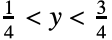
ScalingFunctions (5)
默认情况下,LogLinearPlot 在 x 轴使用 Log 刻度,对 y 轴使用线性刻度:
LogLinearPlot[Cos[x], {x, 0, 20}]LogLinearPlot[3 Cos[x], {x, 0, 20}, ScalingFunctions -> "SignedLog"]用 ScalingFunctions 反转 y 轴坐标的方向:
LogLinearPlot[Cos[x], {x, 0, 20}]LogLinearPlot[Cos[x], {x, 0, 20}, ScalingFunctions -> "Reverse"]{LogLinearPlot[Sec[x], {x, 0, 20}, ScalingFunctions -> "Infinite"], LogLinearPlot[Sec[x], {x, 0, 20}, ScalingFunctions -> {Automatic, "Infinite"}]}LogLinearPlot[Sec[x], {x, 0, 20}, ScalingFunctions -> {Automatic, {Log[#]&, Exp[-#]&}}]应用 (1)
属性和关系 (4)
如果必要的话,LogLinearPlot 会取样更多的点:
LogLinearPlot[Sin[x], {x, 1, 10}, Mesh -> All]LogLinearPlot 是曲线 Plot 的特殊情况:
{LogLinearPlot[Sin[x], {x, 1, 10}], Plot[Sin[Exp[x]], {x, Log[1], Log[10]}, AxesOrigin -> {0, -1}]}使用 LogPlot 和 LogLogPlot 在  方向上画对数图:
LogLogPlot[Abs[10 ^ 2 / ((I ω) ^ 2 + 100)], {ω, 10 ^ 0, 10 ^ 5}]使用 ListLogLinearPlot 处理数据:
{ListLogLinearPlot[Table[{x, Erf[x]}, {x, 0.01, 10, 0.05}], PlotRange -> All], LogLinearPlot[Erf[x], {x, 0.01, 10}]}文本
Wolfram Research (2007),LogLinearPlot,Wolfram 语言函数,https://reference.wolfram.com/language/ref/LogLinearPlot.html (更新于 2026 年).
CMS
Wolfram 语言. 2007. "LogLinearPlot." Wolfram 语言与系统参考资料中心. Wolfram Research. 最新版本 2026. https://reference.wolfram.com/language/ref/LogLinearPlot.html.
APA
Wolfram 语言. (2007). LogLinearPlot. Wolfram 语言与系统参考资料中心. 追溯自 https://reference.wolfram.com/language/ref/LogLinearPlot.html 年