


NyquistPlot
NyquistPlot[lsys]
generates a Nyquist plot of the transfer function for the system lsys.
NyquistPlot[lsys,{ωmin,ωmax}]
plots for the frequency range ωmin to ωmax.
NyquistPlot[expr,{ω,ωmin,ωmax}]
plots expr using the variable ω.
Details and Options


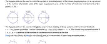
- NyquistPlot gives the complex-plane plot of the transfer function of lsys as the Nyquist contour is traversed.
- The system lsys can be TransferFunctionModel or StateSpaceModel, including descriptor and delay systems.
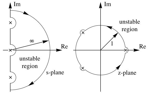
- For continuous-time systems, the Nyquist contour encloses the entire right half-plane and excludes poles on the imaginary axis. It is traversed in a clockwise direction.
- For discrete-time systems, the Nyquist contour is the unit circle, and it encloses poles on the unit circle. It is traversed in a counterclockwise direction.
- The arrows on the NyquistPlot show the direction the Nyquist contour is traversed.
- The Nyquist contours:
- For a system lsys with the corresponding transfer function
 , the following expressions are plotted:
 -

continuous-time system 
discrete-time system with sample time 
- If the frequency range is not specified, the entire Nyquist contour is traversed, effectively
 for continuous-time systems, and
  for discrete-time systems.
 - NyquistPlot treats the variable ω as local, effectively using Block.
- The Nyquist plot can be used to infer the number of unstable poles
 of the closed-loop system as
  , where
  is the number of unstable poles of the open-loop system, and
  is the number of clockwise encirclements of the point
  . »
. » - The Nyquist plot can be used to infer global exponential stability of linear systems with nonlinear feedback
 , where
  satisfies a sector constraint
  when
when  . The closed-loop system is stable if
  , where
  is the number of clockwise encirclements of the disk
 ![TemplateBox[{Disk, paclet:ref/Disk}, RefLink, BaseStyle -> {InlineFormula}][{-(b+a)/(2 a b),0},TemplateBox[{Abs, paclet:ref/Abs}, RefLink, BaseStyle -> {InlineFormula}][(b-a)/(2 a b)]]](Files/NyquistPlot.en/20.png "TemplateBox[{Disk, paclet:ref/Disk}, RefLink, BaseStyle -> {InlineFormula}][{-(b+a)/(2 a b),0},TemplateBox[{Abs, paclet:ref/Abs}, RefLink, BaseStyle -> {InlineFormula}][(b-a)/(2 a b)]]") , and
, and  is the number of open-loop unstable poles. »
 - NyquistPlot has the same options as Graphics, with the following additions and changes: [List of all options]
-
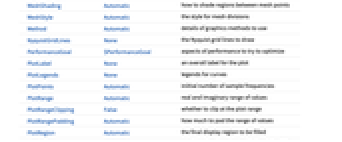
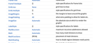
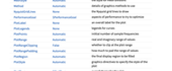
Axes True whether to draw axes ColorFunction Automatic how to apply coloring to the curve ColorFunctionScaling True whether to scale arguments to ColorFunction EvaluationMonitor None expression to evaluate at every evaluation Exclusions True frequencies to exclude ExclusionsStyle Automatic what to draw at excluded frequencies FeedbackSector None the sector limits for feedback function FeedbackSectorStyle Automatic style for feedback sector disk FeedbackType "Negative" the feedback type MaxRecursion Automatic maximum recursive subdivisions allowed Mesh Automatic how many mesh divisions to draw MeshFunctions {#3&} placement of mesh divisions MeshShading Automatic how to shade regions between mesh points MeshStyle Automatic the style for mesh divisions NyquistGridLines None the Nyquist grid lines to draw PerformanceGoal $PerformanceGoal aspects of performance to try to optimize PlotLegends None legends for curves PlotPoints Automatic iniitial number of sample frequencies PlotRange Automatic real and imaginary range of values PlotStyle Automatic graphics directives to specify the style of the plot PlotTheme $PlotTheme overall theme for the plot RegionFunction Automatic how to determine if a point should be included SamplingPeriod None the sampling period StabilityMargins False whether to show the stability margins StabilityMarginsStyle Automatic graphics directives to specify the style of the stability margins WorkingPrecision MachinePrecision the precision used in internal computations - ColorData["DefaultPlotColors",1] gives the default color used by PlotStyle.
- The setting Exclusions->True excludes frequencies, including resonant frequencies, where the sinusoidal transfer function is discontinuous.
- Exclusions->{f1,f2,…} excludes specific frequencies fi.
- ExclusionsStyle->s specifies that style s should be used to render the curve joining opposite ends of each excluded point.
- Points corresponding to exclusions at resonant frequencies are joined by semicircles at infinity.
- FeedbackSector->{a,b} indicates feedback
 with
with  .
. -
AlignmentPoint Center the default point in the graphic to align with AspectRatio Automatic ratio of height to width Axes True whether to draw axes AxesLabel None axes labels AxesOrigin Automatic where axes should cross AxesStyle {} style specifications for the axes Background None background color for the plot BaselinePosition Automatic how to align with a surrounding text baseline BaseStyle {} base style specifications for the graphic ColorFunction Automatic how to apply coloring to the curve ColorFunctionScaling True whether to scale arguments to ColorFunction ContentSelectable Automatic whether to allow contents to be selected CoordinatesToolOptions Automatic detailed behavior of the coordinates tool Epilog {} primitives rendered after the main plot EvaluationMonitor None expression to evaluate at every evaluation Exclusions True frequencies to exclude ExclusionsStyle Automatic what to draw at excluded frequencies FeedbackSector None the sector limits for feedback function FeedbackSectorStyle Automatic style for feedback sector disk FeedbackType "Negative" the feedback type FormatType TraditionalForm the default format type for text Frame False whether to put a frame around the plot FrameLabel None frame labels FrameStyle {} style specifications for the frame FrameTicks Automatic frame ticks FrameTicksStyle {} style specifications for frame ticks GridLines None grid lines to draw GridLinesStyle {} style specifications for grid lines ImageMargins 0. the margins to leave around the graphic ImagePadding All what extra padding to allow for labels etc. ImageSize Automatic the absolute size at which to render the graphic LabelStyle {} style specifications for labels MaxRecursion Automatic maximum recursive subdivisions allowed Mesh Automatic how many mesh divisions to draw MeshFunctions {#3&} placement of mesh divisions MeshShading Automatic how to shade regions between mesh points MeshStyle Automatic the style for mesh divisions Method Automatic details of graphics methods to use NyquistGridLines None the Nyquist grid lines to draw PerformanceGoal $PerformanceGoal aspects of performance to try to optimize PlotLabel None an overall label for the plot PlotLegends None legends for curves PlotPoints Automatic iniitial number of sample frequencies PlotRange Automatic real and imaginary range of values PlotRangeClipping False whether to clip at the plot range PlotRangePadding Automatic how much to pad the range of values PlotRegion Automatic the final display region to be filled PlotStyle Automatic graphics directives to specify the style of the plot PlotTheme $PlotTheme overall theme for the plot PreserveImageOptions Automatic whether to preserve image options when displaying new versions of the same graphic Prolog {} primitives rendered before the main plot RegionFunction Automatic how to determine if a point should be included RotateLabel True whether to rotate y labels on the frame SamplingPeriod None the sampling period StabilityMargins False whether to show the stability margins StabilityMarginsStyle Automatic graphics directives to specify the style of the stability margins Ticks Automatic axes ticks TicksStyle {} style specifications for axes ticks WorkingPrecision MachinePrecision the precision used in internal computations
List of all options
Examples
open all close allBasic Examples (5)
Scope (24)
Basic Uses (11)
Nyquist plot of a continuous-time system:
Nyquist plot of another continuous-time system:
Nyquist plot of a discrete-time system:
Nyquist plot of a continuous-time, transfer-function model:
Discrete-time, transfer-function model:
Nyquist plot of a state-space model:
The Nyquist plots of systems with resonant frequencies have encirclements at infinity:
An improper system with resonant frequencies:
Specify the expression of the sinusoidal transfer function of a system:
Linear System Stability (7)
There are no unstable open-loop poles (![]() ):
):
The plot shows that ![]() is not encircled (
is not encircled (![]() ):
):
Hence the closed-loop system is stable (![]() ); all poles are stable:
); all poles are stable:
Here ![]() , i.e. one unstable pole in the closed-loop system:
, i.e. one unstable pole in the closed-loop system:
The closed-loop system has two unstable poles:
Now ![]() , and
, and ![]() is encircled counterclockwise, so
is encircled counterclockwise, so ![]() , and hence
, and hence ![]() :
:
The closed-loop system has no unstable poles:
For positive feedback, count encirclement around ![]() ; here
; here ![]() ,
, ![]() :
:
There are ![]() unstable poles in the closed-loop system:
unstable poles in the closed-loop system:
A discrete-time system with no unstable poles (![]() ):
):
There are no encirclements of ![]() (
(![]() ):
):
Hence the closed-loop system is stable (![]() ):
):
A stable discrete-time system (![]() ) with positive feedback:
) with positive feedback:
There is one clockwise encirclement of ![]() (
(![]() ) :
) :
The closed-loop system is unstable, with one pole outside the unit circle:
Nonlinear System Stability (6)
Starting with a stable linear system (![]() ):
):
Using feedback ![]() , where
, where ![]() it is also true that
it is also true that ![]() , since the disk is not encircled:
, since the disk is not encircled:
Simulate closed-loop system constant feedback ![]() for
for ![]() :
:
The following stable system (![]() ) has one clockwise encirclement (
) has one clockwise encirclement (![]() ) of the disk for feedback in the sector
) of the disk for feedback in the sector ![]() :
:
Hence the closed-loop system is unstable for any feedback in that sector:
With a feedback configuration that has one counterclockwise encirclement (![]() ):
):
The closed-loop system is stable with any feedback in the sector:
A stable system has feedback in the sector ![]() , and its NyquistPlot is to the right of
, and its NyquistPlot is to the right of ![]() :
:
The closed loop is stable for any feedback in the sector ![]() :
:
The NyquistPlot lies within the circle for feedback in the sector ![]() :
:
The closed loop is stable for any feedback within the sector ![]() :
:
A stable system lsys with feedback in the sector ![]() :
:
The NyquistPlot of -lsys with feedback in the sector ![]() shows a stable closed-loop system:
shows a stable closed-loop system:
Generalizations & Extensions (1)
Options (58)
AspectRatio (4)
By default, the ratio of the height to width for the plot is determined automatically:
Make the height the same as the width with AspectRatio1:
Use numerical value to specify the height-to-width ratio:
AspectRatioFull adjusts the height and width to tightly fit inside other constructs:
Axes (3)
AxesLabel (4)
No axes labels are drawn by default:
Use labels based on variables specified in NyquistPlot:
AxesOrigin (2)
AxesStyle (4)
CoordinatesToolOptions (1)
Exclusions (5)
ExclusionsStyle (2)
FeedbackSector (4)
ImageSize (7)
Use named sizes such as Tiny, Small, Medium and Large:
Specify the width of the plot:
Specify the height of the plot:
Allow the width and height to be up to a certain size:
Specify the width and height for a graphic, padding with space if necessary:
Setting AspectRatioFull will fill the available space:
Use maximum sizes for the width and height:
Use ImageSizeFull to fill the available space in an object:
Specify the image size as a fraction of the available space:
NyquistGridLines (2)
PlotLegends (4)
Use placeholder legends for multiple systems:
Use the systems as the legend text:
Use LineLegend to add an overall legend label:
PlotRange (2)
Specify the range of coordinates to include in a plot:
Points at infinity are shown in the region specified by PlotRangePadding:
StabilityMargins (2)
Ticks (4)
Applications (2)
Text
Wolfram Research (2010), NyquistPlot, Wolfram Language function, https://reference.wolfram.com/language/ref/NyquistPlot.html (updated 2014).
CMS
Wolfram Language. 2010. "NyquistPlot." Wolfram Language & System Documentation Center. Wolfram Research. Last Modified 2014. https://reference.wolfram.com/language/ref/NyquistPlot.html.
APA
Wolfram Language. (2010). NyquistPlot. Wolfram Language & System Documentation Center. Retrieved from https://reference.wolfram.com/language/ref/NyquistPlot.html