

SinghMaddalaDistribution
SinghMaddalaDistribution[q,a,b]
represents the Singh–Maddala distribution with shape parameters q and a and scale parameter b.
Details
- SinghMaddalaDistribution is also known as Burr XII distribution.
- The probability density for value
 in a Singh–Maddala distribution is proportional to
  for
for  .
. - SinghMaddalaDistribution allows q, a, and b to be any positive real numbers.
- SinghMaddalaDistribution allows b to be a quantity of any unit dimension, and q and a to be dimensionless quantities. »
- SinghMaddalaDistribution can be used with such functions as Mean, CDF, and RandomVariate.
Background & Context
- SinghMaddalaDistribution[q,a,b] represents a continuous statistical distribution supported on the interval
 and parametrized by positive real numbers q, a, and b (two "shape parameters" and a "scale parameter", respectively) that together determine the overall behavior of its probability density function (PDF). Depending on the values of q, a, and b, the PDF of a Singh–Maddala distribution may have any of a number of shapes including unimodal with a single "peak" (i.e. a global maximum) or monotone decreasing with potential singularities approaching the lower boundary of its domain. In addition, the tails of the PDF are "fat" in the sense that the PDF decreases algebraically rather than exponentially for large values of
  . (This behavior can be made quantitatively precise by analyzing the SurvivalFunction of the distribution.) The Singh–Maddala distribution is also sometimes referred to as the Burr XII distribution or as the Burr distribution and is one of a number of distributions referred to as generalized log-logistic distributions (not to be confused with LogLogisticDistribution).
 - The Singh–Maddala distribution was first discovered in the early 1940s by I. W. Burr before being rediscovered in the 1970s by S. K. Singh and G. S. Maddala as an alternative to the gamma (GammaDistribution) and log-normal distributions (LogNormalDistribution) in modeling income distribution. Since then, the Singh–Maddala distribution has been used ubiquitously throughout economics and econometrics to model various financial phenomena and has also been used as a tool in areas such as actuarial science, Monte Carlo theory, publishing, and sociology.
- RandomVariate can be used to give one or more machine- or arbitrary-precision (the latter via the WorkingPrecision option) pseudorandom variates from a Singh–Maddala distribution. Distributed[x,SinghMaddalaDistribution[q,a,b]], written more concisely as xSinghMaddalaDistribution[q,a,b], can be used to assert that a random variable x is distributed according to a Singh–Maddala distribution. Such an assertion can then be used in functions such as Probability, NProbability, Expectation, and NExpectation.
- The probability density and cumulative distribution functions for Singh–Maddala distributions may be given using PDF[SinghMaddalaDistribution[q,a,b],x] and CDF[SinghMaddalaDistribution[q,a,b],x]. The mean, median, variance, raw moments, and central moments may be computed using Mean, Median, Variance, Moment, and CentralMoment, respectively.
- DistributionFitTest can be used to test if a given dataset is consistent with a Singh–Maddala distribution, EstimatedDistribution to estimate a Singh–Maddala parametric distribution from given data, and FindDistributionParameters to fit data to a Singh–Maddala distribution. ProbabilityPlot can be used to generate a plot of the CDF of given data against the CDF of a symbolic Singh–Maddala distribution, and QuantilePlot to generate a plot of the quantiles of given data against the quantiles of a symbolic Singh–Maddala distribution.
- TransformedDistribution can be used to represent a transformed Singh–Maddala distribution, CensoredDistribution to represent the distribution of values censored between upper and lower values, and TruncatedDistribution to represent the distribution of values truncated between upper and lower values. CopulaDistribution can be used to build higher-dimensional distributions that contain a Singh–Maddala distribution, and ProductDistribution can be used to compute a joint distribution with independent component distributions involving Singh–Maddala distributions.
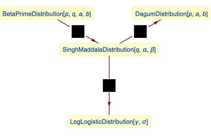
- SinghMaddalaDistribution is related to a number of other distributions. SinghMaddalaDistribution generalizes LogLogisticDistribution (the PDF of SinghMaddalaDistribution[1,γ,σ] is precisely that of LogLogisticDistribution[γ,σ]), is generalized by BetaPrimeDistribution (the PDF of SinghMaddalaDistribution[q,a,b] is exactly that of BetaPrimeDistribution[1,q,a,b]), and is a transformation (TransformedDistribution) of DagumDistribution. SinghMaddalaDistribution is also closely related to BetaDistribution, ParetoDistribution, PearsonDistribution, GammaDistribution, WeibullDistribution, and LogNormalDistribution.
Examples
open all close allBasic Examples (4)
Plot[Table[PDF[SinghMaddalaDistribution[2, a, 3], x], {a, {1, 2.5, 5}}]//Evaluate, {x, 0, 6}, PlotRange -> All, Filling -> Axis]Plot[Table[PDF[SinghMaddalaDistribution[q, 2, 3], x], {q, {0.5, 1.5, 4}}]//Evaluate, {x, 0, 6}, PlotRange -> All, Filling -> Axis]Plot[Table[PDF[SinghMaddalaDistribution[.5, 1.5, b], x], {b, {1, 2, 3}}]//Evaluate, {x, 0, 5}, PlotRange -> All, Filling -> Axis]PDF[SinghMaddalaDistribution[q, a, b], x]Cumulative distribution function:
Plot[Table[CDF[SinghMaddalaDistribution[2, a, 3], x], {a, {1, 2.5, 5}}]//Evaluate, {x, 0, 6}, PlotRange -> All, Filling -> Axis]Plot[Table[CDF[SinghMaddalaDistribution[q, 2, 3], x], {q, {0.5, 1.5, 4}}]//Evaluate, {x, 0, 6}, PlotRange -> All, Filling -> Axis]Plot[Table[CDF[SinghMaddalaDistribution[.5, 1.5, b], x], {b, {1, 2, 3}}]//Evaluate, {x, 0, 5}, PlotRange -> All, Filling -> Axis]CDF[SinghMaddalaDistribution[q, a, b], x]Mean and variance may not be defined for all parameter values:
Mean[SinghMaddalaDistribution[q, a, b]]Variance[SinghMaddalaDistribution[q, a, b]]Median[SinghMaddalaDistribution[q, a, b]]Scope (8)
Generate a sample of pseudorandom numbers from a Singh–Maddala distribution:
data = RandomVariate[SinghMaddalaDistribution[3, 2.2, 5], 10 ^ 4];Compare its histogram to the PDF:
Show[
	Histogram[data, {0, 10, 1 / 2}, "PDF"],
	Plot[PDF[TruncatedDistribution[{0, 10}, SinghMaddalaDistribution[3, 2.2, 5]], x], {x, 0, 10}, PlotStyle -> Thick]]
Distribution parameters estimation:
sample = RandomVariate[SinghMaddalaDistribution[2, 3, 4], 10 ^ 3];Estimate the distribution parameters from sample data:
edist = EstimatedDistribution[sample, SinghMaddalaDistribution[q, a, b]]Compare the density histogram of the sample with the PDF of the estimated distribution:
Show[Histogram[sample, {0, 10, 0.5}, "PDF"], Plot[PDF[edist, x], {x, 0, 10}, PlotStyle -> Thick]]Skewness varies with the shape parameters ![]() and
and ![]() and is defined when
and is defined when ![]() :
:
Plot3D[Skewness[SinghMaddalaDistribution[q, a, 2]], {a, 4, 8}, {q, 1, 3}, MeshFunctions -> {#3&}, MeshShading -> ColorData[35, "ColorList"], AxesLabel -> Automatic]Skewness[SinghMaddalaDistribution[q, a, b]]Plot3D[Kurtosis[SinghMaddalaDistribution[q, a, 2]], {a, 4, 8}, {q, 1, 3}, MeshFunctions -> {#3&}, MeshShading -> ColorData[35, "ColorList"], AxesLabel -> Automatic]Kurtosis[SinghMaddalaDistribution[q, a, b]]Different moments with closed forms as functions of parameters:
FormulaGrid[list_, type_] := Grid[...]FormulaGrid[Table[Moment[SinghMaddalaDistribution[q, a, b], k], {k, 3}], M]Closed form for symbolic order:
Moment[SinghMaddalaDistribution[q, a, b], r]FormulaGrid[Table[CentralMoment[SinghMaddalaDistribution[q, a, b], k], {k, 3}], CM]FormulaGrid[Table[FactorialMoment[SinghMaddalaDistribution[q, a, b], k], {k, 3}], FM]FormulaGrid[Table[Cumulant[SinghMaddalaDistribution[q, a, b], k], {k, 3}], C]Plot[Table[HazardFunction[SinghMaddalaDistribution[q, 1.5, 2], x], {q, {0.5, 1, 2}}]//Evaluate, {x, 0, 6}, Filling -> Axis]Plot[Table[HazardFunction[SinghMaddalaDistribution[2, 1.5, b], x], {b, {1, 2, 4}}]//Evaluate, {x, 0, 6}, Filling -> Axis]Plot[Table[HazardFunction[SinghMaddalaDistribution[2, a, 1.5], x], {a, {1, 2, 3}}]//Evaluate, {x, 0, 6}, Filling -> Axis]HazardFunction[SinghMaddalaDistribution[q, a, b], x]Plot[Table[Quantile[SinghMaddalaDistribution[q, 2, 1.3], z], {q, {1, 3, 8}}]//Evaluate, {z, 0, 1}, Filling -> Axis]Plot[Table[Quantile[SinghMaddalaDistribution[2, a, 1.3], z], {a, {1, 3, 10}}]//Evaluate, {z, 0, 1}, Filling -> Axis]Plot[Table[Quantile[SinghMaddalaDistribution[2, 5, b], z], {b, {1, 3, 5}}]//Evaluate, {z, 0, 1}, Filling -> Axis]Quantile[SinghMaddalaDistribution[q, a, b], z]Consistent use of Quantity in parameters yields QuantityDistribution:
earthquake𝒟 = SinghMaddalaDistribution[0.47, 5.64, Quantity[35.1, IndependentUnit["Earthquakes"]]]Quartiles[earthquake𝒟]Applications (1)
The number of earthquakes per year can be modeled with SinghMaddalaDistribution:
ExampleData[{"Statistics", "USEarthquakes"}, "LongDescription"]earthquakes = Counts[
Cases[ExampleData[{"Statistics", "USEarthquakes"}], {year_ /; year ≥ 1935, __} :> year]]Fit the distribution to the data:
edist = EstimatedDistribution[earthquakes//Values, SinghMaddalaDistribution[q, a, b]]Compare the data histogram with the PDF of the estimated distribution:
Show[Histogram[earthquakes, 15, "PDF"], Plot[PDF[edist, x], {x, 0, 140}, PlotStyle -> Thick]]Find the probability of at least 60 earthquakes in the US in a year:
NProbability[x ≥ 60, xedist]Find the mean amount of earthquakes in the US in a year:
Mean[edist]Simulate the number of earthquakes per year for the next 30 years:
ListPlot[{RandomVariate[edist, 30], {{0, Mean[edist]}, {30, Mean[edist]}}}, Joined -> {False, True}, Filling -> Axis, AxesOrigin -> {0, 0}, PlotRange -> All]Properties & Relations (8)
Singh–Maddala distribution is closed under scaling by a positive factor:
TransformedDistribution[k * u, uSinghMaddalaDistribution[q, a, b]]The family of SinghMaddalaDistribution is closed under a minimum:
OrderDistribution[{SinghMaddalaDistribution[q, a, b], n}, 1]TransformedDistribution[Min[x, y], {xSinghMaddalaDistribution[Subscript[q, 1], a, b], ySinghMaddalaDistribution[Subscript[q, 2], a, b]}]The hazard function is unimodal for ![]() , and decreasing for
, and decreasing for ![]() :
:
Plot[Table[Legended[HazardFunction[SinghMaddalaDistribution[.5, a, 1.5], x], Row[{"a = ", a}]], {a, 0.2, 2, 0.5}]//Evaluate, {x, 0, 6}]The parameter q is a scale factor for the hazard function:
Plot[Table[Legended[HazardFunction[SinghMaddalaDistribution[q, 1.5, 1.5], x], Row[{"q = ", q}]], {q, 1, 4}]//Evaluate, {x, 0, 6}]Relations to other distributions:
SinghMaddalaDistribution is a special case of BetaPrimeDistribution:
PDF[SinghMaddalaDistribution[q, a, b], x]PDF[BetaPrimeDistribution[1, q, a, b], x]//FullSimplifyFullSimplify[% - %%, a > 0 && b > 0]If ![]() has a SinghMaddalaDistribution, then
has a SinghMaddalaDistribution, then ![]() has a DagumDistribution:
has a DagumDistribution:
TransformedDistribution[1 / x, xSinghMaddalaDistribution[q, a, b]]LogLogisticDistribution is a special case of SinghMaddalaDistribution:
PDF[SinghMaddalaDistribution[1, γ, σ], x]PDF[LogLogisticDistribution[γ, σ], x]% - %%Neat Examples (1)
PDFs for different q values with CDF contours:
dist = SinghMaddalaDistribution[q, 2, 3];cdf = Function[{x, q}, Evaluate[CDF[dist, x]]];
ql = {0.025, 0.10, 0.25, 0.5, 0.75, 0.90, 0.975};
cl = Table[ColorData["Rainbow"][q], {q, Join[{0.0}, ql]}];Legended[Plot3D[PDF[dist, x], {x, 0, 6}, {q, 0.2, 3}, PlotTheme -> "Marketing", MeshFunctions -> {cdf}, Mesh -> {ql}, MeshStyle -> GrayLevel[0.8], MeshShading -> cl, AxesLabel -> Automatic, BaseStyle -> Opacity[0.9], ImageSize -> 400, PlotRange -> All, PlotPoints -> 50], BarLegend["Rainbow", ql, LegendLabel -> "prob"]]Text
Wolfram Research (2010), SinghMaddalaDistribution, Wolfram Language function, https://reference.wolfram.com/language/ref/SinghMaddalaDistribution.html (updated 2016).
CMS
Wolfram Language. 2010. "SinghMaddalaDistribution." Wolfram Language & System Documentation Center. Wolfram Research. Last Modified 2016. https://reference.wolfram.com/language/ref/SinghMaddalaDistribution.html.
APA
Wolfram Language. (2010). SinghMaddalaDistribution. Wolfram Language & System Documentation Center. Retrieved from https://reference.wolfram.com/language/ref/SinghMaddalaDistribution.html