NIntegrate 积分规则
介绍
积分规则通常使用加权和对一个区域上的积分进行估值. 对于 NIntegrate 的用法而言,一个积分规则对象既进行积分估计,也进行误差估计,作为积分估计准确性的测量手段.
下面的一般说明与诸如 "GaussKronrodRule" 和 "MultidimensionalRule" 一类的加权总和类型积分规则相关. 适用于 "LevinRule" 等其它类型的规则另有单独的讨论.
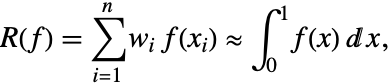
积分规则在一组点上对被积函数进行采样,这些点称为采样点. 在文献中这些也称为横坐标. 与每一个采样点  相对应,有一个权重数
 . 积分规则根据加权和
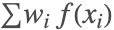 估计积分
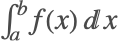 . 积分规则是一个泛函,也就是说,它在区间
 (或一个更一般的区域)上将函数映射到实数.


对于以下讨论的规则,对积分进行估值的取样点选取于区间  、单位立方体
 或者是位于中心的单位立方体
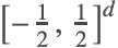 ,其中
 是积分的维数. 所以如果
 是这样一个区域,则使用
 而不是
 . 当这些规则应用于其它区域时,其横坐标和估计值需要相应地进行缩放.



一个积分规则  在一个函数
 中的应用将被视为
 的一个积分,例如,“当
 被
 积时,得到
 ."
对于一个一维积分规则,如果被积多项式的次数都小于或等于  ,并且对于至少一个次数为
 的多项式会失败,则称这个一维积分规则的次数为
 .
对于一个多维积分规则,如果被积单项式的次数都小于或等于  ,并且对于至少一个次数为
 的单项式会失败,则称这个多维积分规则的次数为
 ,也就是说,对于所有形如
 的单项式,积分规则是准确的,其中
 为维数,
 ,且
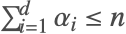 .
一个次数为  的空规则对于所有次数
 的单项式的积分为零,且对于对于至少一个次数为
 的单项式会失败. 每一个空规则可以被视作一个基本积分规则与一个次数较低的适当积分规则的差.
如果次数为  的规则
 的样本点集包含一个次数为
 的规则的
 样本点集,且
 ,则称
 嵌入
 ,并记作
 .
如果次数为  的积分规则是具有共同推导和性能但不同次数的一个规则族的成员,则被记作
 ,其中
 可能被选出对规则族进行标识. (例如,4次梯形规则可以被称为
 .)
如果在一个族中的每一个规则都是该族中另一个规则的嵌入,则称该族的规则是渐进的. (对于任意  ,存在
 ,满足
 ).
如果被积函数在区间的两个端点不进行计算,则称这个积分规则是开放型的. 如果在区间端点计算被积函数则称之为封闭型.
一个 NIntegrate 积分规则对象对于积分估计有一个积分规则,对于误差估计有一个或几个空规则. 积分规则和空规则的样本点是一致的. 根据上下文应该判断出“积分规则”或“规则”指的是一个 NIntegrate 积分规则对象,还是通常数学意义上的一个积分规则.
积分规则规范
下述所有的积分规则,除了 "MonteCarloRule" 以外,都将用于NIntegrate 的自适应策略. 在NIntegrate 中,包括原始和自适应的所有蒙特卡洛策略都使用 "MonteCarloRule".
在 NIntegrate 中的自适应策略所用的积分规则(见 "全局自适应策略" 和 "局部自适应策略")是通过 Method 子选项指定的.
NIntegrate[1 / Sqrt[x], {x, 0, 1}, Method -> {"GlobalAdaptive", Method -> "ClenshawCurtisRule"}]//InputFormNIntegrate[1 / Sqrt[x], {x, 0, 1}, Method -> {"LocalAdaptive", Method -> "ClenshawCurtisRule"}]//InputForm如果 NIntegrate 给出的方法选项只有一个不为 "MonteCarloRule" 的积分规则规范,则该规则与 "GlobalAdaptive" 策略结合使用. 下面的两个输入是等价的.
NIntegrate[1 / Sqrt[x], {x, 0, 1}, Method -> "LobattoKronrodRule"]//InputFormNIntegrate[1 / Sqrt[x], {x, 0, 1}, Method -> {"GlobalAdaptive", Method -> "LobattoKronrodRule"}]//InputForm对于 "MonteCarloRule",自动使用自适应蒙特卡洛策略. 下面两个命令是等价的.
NIntegrate[1 / Sqrt[x], {x, 0, 1}, Method -> "MonteCarloRule"]//InputFormNIntegrate[1 / Sqrt[x], {x, 0, 1}, Method -> {"AdaptiveMonteCarlo", Method -> "MonteCarloRule"}]//InputForm"TrapezoidalRule"
积分估计的梯形规则是最简单也是最古老的规则之一(可能曾被巴比伦人使用,但一定曾被古希腊数学家使用):



如果选项 Method 的值为 "TrapezoidalRule",则复合梯形规则被用来估计由积分策略形成的每一个子区间.
NIntegrate[x + 5, {x, 0, 7}, Method -> "TrapezoidalRule"]选项名称 | 默认值 | |
| "Points" | 5 | 粗略梯形点数 |
| "RombergQuadrature" | True | 是否使用 Romberg 求积法 |
| "SymbolicProcessing" | Automatic | 进行符号预处理的秒数 |
梯形规则及其复合(多面板)扩展并不十分准确. (复合梯形规则对于线性函数是准确的,并且如果被积函数的二阶导数连续,则至少以  的速度收敛 [DavRab84].)多面板梯形规则的准确度可以通过使用 Romberg 求积法 提高.
由于  的横坐标是
 的子集,差值
 可用作积分估计
 的误差估计,且不用额外计算被积函数就可求出.
选项 "Points"->k 可用来指定粗略点的个数. "TrapezoidalRule" 所用的总点数为  .
k = 4;
Reap@NIntegrate[x + 5, {x, 1, 7}, Method -> {"TrapezoidalRule", "Points" -> k, "RombergQuadrature" -> False}, EvaluationMonitor :> Sow[x]]
NIntegrate[x ^ 2 + y, {x, 0, 1}, {y, 0, 1}, Method -> "TrapezoidalRule"]评注:NIntegrate 既有梯形规则也有梯形策略;见教程“积分策略”中的" 'Trapezoidal' 策略". 所有 NIntegrate 的内部执行的规则都有后缀 -Rule. 因此 "TrapezoidalRule" 用于指定梯形积分规则,"Trapezoidal" 用于指定梯形策略.
Romberg 求积法
Romberg 求积法的思想是使用  和
 的线性组合消去
 和
 的截断近似误差的阶数相同的项.
根据 Euler–Maclaurin 公式 [DavRab84],有

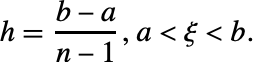


如果从第二个方程中减去第一个方程4次,可以消去上述方程中的  项. 结果是


NIntegrate[Sqrt[x], {x, 0, 1}, Method -> {"GlobalAdaptive", Method -> {"TrapezoidalRule", "Points" -> 5, "RombergQuadrature" -> True}, "SingularityDepth" -> ∞}, MaxRecursion -> 100, PrecisionGoal -> 8]//InputForm//TimingNIntegrate[Sqrt[x], {x, 0, 1}, Method -> {"GlobalAdaptive", Method -> {"TrapezoidalRule", "Points" -> 5, "RombergQuadrature" -> False}, "SingularityDepth" -> ∞}, MaxRecursion -> 100, PrecisionGoal -> 8]//InputForm//Timing"TrapezoidalRule" 采样点和权重
n = 5;precision = MachinePrecision;
{absc, weights, errweights} = NIntegrate`TrapezoidalRuleData[n, precision]rombergAbsc = absc;
lowOrderWeights = -(errweights - weights);
rombergWeights = (4weights - lowOrderWeights/3);
rombergErrorWeights = rombergWeights - weights;
{rombergAbsc, rombergWeights, rombergErrorWeights}"NewtonCotesRule"
Newton–Cotes 积分公式是有相同间隔采样点的插值型公式.
NIntegrate[1 / Sqrt[x], {x, 0, 1}, Method -> "NewtonCotesRule"]选项名称 | 默认值 | |
| "Points" | 3 | 粗略 Newton–Cotes 点数 |
| "Type" | Closed | Newton–Cotes 规则的类型 |
| "SymbolicProcessing" | Automatic | 进行符号预处理的秒数 |






当  很大时,Newton–Cotes
 点系数也很大并且符号混合.
NIntegrate`NewtonCotesRuleData[25, MachinePrecision][[2]]由于相互抵消,可能导致大量有效数位的丢失,因此使用高阶 Newton–Cotes 规则时必须谨慎.
"NewtonCotesRule" 采样点和权重
n = 5;precision = MachinePrecision;
{absc, weights, errweights} = NIntegrate`NewtonCotesRuleData[n, precision]
"GaussBerntsenEspelidRule"
高斯求积法使用最佳采样点(通过多项式插值法得到)形成在这些点上的被积函数值的加权和. 在这些采样点的子集上,可以使用一个较低阶的求积法规则. 两个规则的差可用来进行误差估计. Berntsen 和 Espelid 通过去除奇数个采样点的高斯规则的中点推导得到了误差估计规则.
NIntegrate[1 / Sqrt[x], {x, 0, 1}, Method -> "GaussBerntsenEspelidRule"]"GaussBerntsenEspelidRule" 选项.
对被积函数  ,
 个点的高斯规则
 对于次数为
 的多项式是准确的(也就是说,若
 为次数为
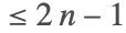 的多项式,则
 ).
由于不计算被积函数在区间两个端点处的值,因此高斯规则是开放型的. (Lobatto 规则, Clenshaw–Curtis 规则和梯形规则 是封闭型的,因为它们计算被积函数在区间端点处的值.)
这里定义了差商泛函 [Ehrich2000]

对于采样点为  的高斯规则
 ,Berntsen 和 Espelid 已推导得到了下面的误差估计函数(error estimate functional)(see [Ehrich2000])

([Ehrich2000] 中的原始公式针对的是区间  上的采样点. 上述公式针对的是区间
 上的采样点.)
Table[(k = 0;NIntegrate[x ^ (1 / 2), {x, 0, 1}, Method -> {"GaussBerntsenEspelidRule", "Points" -> i}, EvaluationMonitor :> k++];k), {i, 2, 20}]"GaussBerntsenEspelidRule" 采样点和权重
n = 5;precision = 20;
{absc, weights, errweights} = NIntegrate`GaussBerntsenEspelidRuleData[n, precision]polyd[vec_List, nu_] := (Times@@(vec[[nu]] - Drop[vec, {nu}])) ^ (-1);
dvdWeights[vec_List] := dvdWeights[vec] = Table[polyd[vec, nu], {nu, 1, Length[vec]}];
{absc, weights, errweights} = NIntegrate`GaussRuleData[2n + 1, precision];(((-1)^n Sqrt[π] Gamma[1 + n]^2)/Gamma[(3/2) + 2 n] 2^2 n) dvdWeights[absc]"GaussKronrodRule"
高斯求积法使用最佳采样点(通过多项式插值得到)来形成在这些点处被积函数值的加权和. 高斯规则的 Kronrod 扩展是在高斯点之间增加新采样点而形成一个更高阶的规则,而该规则重新使用高斯规则被积函数的计算方法.
NIntegrate[1 / Sqrt[x], {x, 0, 1}, Method -> "GaussKronrodRule"]对被积函数  ,
 个点的高斯规则
 对于次数为
 的多项式是准确的,也就是说,若
 为次数为
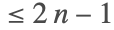 的多项式,则
 ).
由于不计算被积函数在区间两个端点处的值,因此高斯–Kronrod 规则是开放型的.
具有  个点的高斯规则
 的 Kronrod 扩展
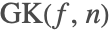 对
 增加
 个点. 扩展的规则对于次数为
 (
 为偶数)或
 (
 为奇数)的多项式是准确的. 与高斯规则相关的权重在其 Kronrod 扩展中会改变.
由于  的横坐标是
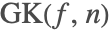 的一个子集,差值
 可用于表示积分估计
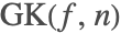 的一个误差估计,可以在不用额外计算被积函数的情况下被计算.
Table[(k = 0;NIntegrate[x ^ 10, {x, 0, 1}, Method -> {"GaussKronrodRule", "Points" -> i}, EvaluationMonitor :> k++];k), {i, 2, 20}]关于高斯规则的 Kronrod 扩展的执行介绍,请见[PiesBrand74].
"GaussKronrodRule" 采样点和权重
n = 5;precision = 20;
{absc, weights, errweights} = NIntegrate`GaussKronrodRuleData[n, precision]
下面的计算显示出高斯-Kronrod 积分规则的次数(见上).
p = If[OddQ[n], 3 * n + 2, 3 * n + 1]f[x_] := x^p下面的命令执行了积分估计 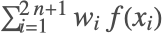 和误差估计
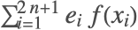 的积分规则加权和,其中
 是横坐标,
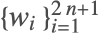 是权重,
 是误差权重.

Total@MapThread[{f[#1]#2, f[#1]#3}&, {absc, weights, errweights}]N[Integrate[f[x], {x, 0, 1}], precision]该误差估计非零,原因是嵌入的高斯规则对于次数 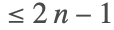 的多项式是准确的. 如果对这样次数的多项式进行积分,则误差估计为零.
f[x_] := x^2n - 1
Total@MapThread[{f[#1]#2, f[#1]#3}&, {absc, weights, errweights}]N[Integrate[f[x], {x, 0, 1}], precision]"LobattoKronrodRule"
Lobatto 积分规则是一种预先对横坐标赋值的高斯型规则. 它使用积分区间端点和区间内的最佳采样点来形成在这些点上被积函数值的加权和. Lobatto 规则的 Kronrod 扩展是在Lobatto 规则点之间增加新采样点而形成一个更高阶的规则,而该规则重新使用 Lobatto 规则被积函数的计算方法.
NIntegrate[1 / Sqrt[x], {x, 0, 1}, Method -> "LobattoKronrodRule"]选项名称 | 默认值 | |
| "Points" | 5 | 与 Kronrod 点一起被扩展的高斯–Lobatto 点的个数 |
| "SymbolicProcessing" | Automatic | 进行符号预处理的秒数 |
对被积函数  ,
 个点的 Lobatto 规则
 对于次数为
 的多项式是准确的,也就是说,若
 为次数为
 的多项式,则
 ).
具有  个点的 Lobatto 规则
 的 Kronrod 扩展
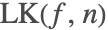 对
 增加了
 个点,扩展了的规则对于次数为
 (
 为偶数)或
 (
 为奇数)的多项式是准确的. 与 Lobatto 规则相关的权重在其 Kronrod 扩展中会变化.
与 "GaussKronrodRule" 相同,选项 "GaussPoints" 设定高斯点的个数. 如果 "LobattoKronrodRule" 被"Points"->n 激活,则规则点的总个数为  .
Table[(k = 0;NIntegrate[x ^ 10, {x, 0, 1}, Method -> {"LobattoKronrodRule", "Points" -> i}, EvaluationMonitor :> k++];k), {i, 3, 20}]由于 Lobatto 规则 是封闭型的,需要计算区间端点的被积函数值. 如果在这些端点处有奇点,则将被 NIntegrate 忽略.
关于 Lobatto 规则的 Kronrod 扩展的执行介绍,请见[PiesBrand74].
"LobattoKronrodRule" 采样点和权重
n = 5;precision = 20;
{absc, weights, errweights} = NIntegrate`LobattoKronrodRuleData[n, precision]
下面的计算显示了 Lobatto–Kronrod 积分规则的次数( 见上).
p = If[OddQ[n], 3 * n - 3, 3 * n - 2]f[x_] := x^p下面的命令执行了积分估计 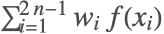 和误差估计
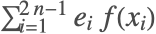 的积分规则加权和,其中
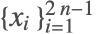 是横坐标,
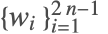 是权重,
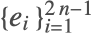 是误差权重.

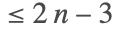
Total@MapThread[{f[#1]#2, f[#1]#3}&, {absc, weights, errweights}]N[Integrate[f[x], {x, 0, 1}], precision]上面的误差估计非零,原因是嵌入的 Lobatto 规则对于次数 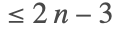 的多项式是准确的. 如果对这样次数的多项式进行积分,则误差估计为零.
f[x_] := x^2n - 3
Total@MapThread[{f[#1]#2, f[#1]#3}&, {absc, weights, errweights}]N[Integrate[f[x], {x, 0, 1}], precision]"ClenshawCurtisRule"
Clenshaw–Curtis 规则使用的采样点是通过被积函数的切比雪夫多项式近似得到的.
NIntegrate[1 / Sqrt[x], {x, 0, 1}, Method -> "ClenshawCurtisRule"]选项名称 | 默认值 | |
| "Points" | 5 | 粗略 Clenshaw–Curtis 点的个数 |
| "SymbolicProcessing" | Automatic | 进行符号预处理的秒数 |
理论上一个具有  个采样点的 Clenshaw–Curtis规则对于次数等于或小于
 的多项式是准确的. 然而实际上Clenshaw–Curtis 规则能达到高斯规则 [Evans93][OHaraSmith68] 的准确度. Clenshaw–Curtis 公式的误差分析请见 [OHaraSmith68].
经典 Clenshaw–Curtis 规则的采样点是切比雪夫多项式的零点 .实用 Clenshaw–Curtis 规则的采样点是切比雪夫多项式的极值点. 经典 Clenshaw–Curtis 规则不是渐进的,但实用 Clenshaw–Curtis 规则是 [DavRab84][KrUeb98].
令 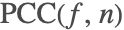 代表函数
 的
 个采样点的一个实用 Clenshaw–Curtis 规则.
渐进性质意味着 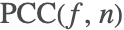 的采样点是
 的采样点的子集. 因此差值
 可用于表示积分估计
 的一个误差估计,可以在不用额外计算被积函数的情况下被计算.


NIntegrate[Sqrt[x], {x, 0, 1}, Method -> {"ClenshawCurtisRule", "Points" -> 10}]Table[(k = 0;NIntegrate[x ^ 10, {x, 0, 1}, Method -> {"ClenshawCurtisRule", "Points" -> i}, EvaluationMonitor :> k++];k), {i, 3, 20}]"ClenshawCurtisRule" 采样点和权重
n = 5;precision = 20;
{absc, weights, errweights} = NIntegrate`ClenshawCurtisRuleData[n, precision]
nn = 2n - 1;
N[(1/2)Table[Cos[(π/nn - 1)i], {i, nn - 1, 0, -1}] + (1/2), precision]f[x_] := x^2n - 1
Total@MapThread[{f[#1]#2, f[#1]#3}&, {absc, weights, errweights}]Integrate[f[x], {x, 0, 1}]"MultipanelRule"
"MultipanelRule" 在两个或两个以上的相邻区间上将一维积分规则的应用合并至一个规则中. 在任何一个相邻区间上的原始规则的应用被称为一个面板.
NIntegrate[1 / Sqrt[x], {x, 0, 1}, Method -> {"MultipanelRule", Method -> "GaussKronrodRule", "Panels" -> 3}]选项名称 | 默认值 | |
| Method | "NewtonCotesRule" | 为一个单面板提供横坐标、权重和误差权重的积分规则设定 |
| "Panels" | 5 | 面板个数 |
| "SymbolicProcessing" | Automatic | 进行符号处理需要的秒数 |



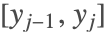



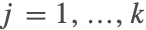



若  是封闭的,即
 存在
 和
 作为采样点,则
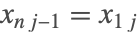 ,且
 的采样点个数可减至
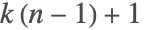 . (这通过执行 "MultipanelRule" 完成.)
更多关于多面板规则的理论(也被称为复合规则),请见 [KrUeb98] 和 [DavRab84].
"MultipanelRule" 采样点和权重
npanels = 3;
NIntegrate`MultiPanelRuleData[{"GaussKronrodRule", "Points" -> 2}, npanels, MachinePrecision]{absc, weights, errweights} = NIntegrate`GaussKronrodRuleData[2, MachinePrecision]Join@@Map[Rescale[absc, {0, 1}, #]&, Partition[Range[0, npanels](1/npanels), 2, 1]](1/npanels)Join@@Table[weights, {npanels}]"CartesianRule"
一个  维 Cartesian 规则的采样点是
 个一维规则的采样点的 Cartesian 乘积. 与 Cartesian 规则的采样点相关的权重是对应于其坐标的一维规则权重的乘积.
NIntegrate[1 / Sqrt[x + y + z], {x, 0, 1}, {y, 0, 1}, {z, 0, 1}, Method -> "CartesianRule"]选项名称 | 默认值 | |
| Method | "GaussKronrodRule" | 形成 Cartesian 乘积规则的一个规则或规则列表 |
| "SymbolicProcessing" | Automatic | 进行符号预处理需要的秒数 |
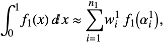
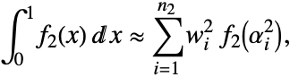
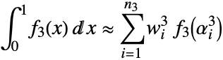
这些公式分别对次数为  、
 和
 的多项式是准确的. 则不难看出
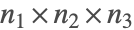 个点的公式

对于次数为  的
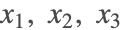 中的多项式是准确的. 注意与横坐标
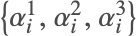 相关的权重是
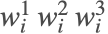 .
对  个一维规则(其中
 个规则有
 个采样点
 和权重
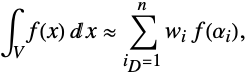
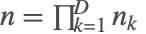
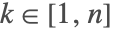
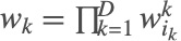
 ),其一般 Cartesian 乘积公式是




pnts = Reap[NIntegrate[x + y ^ 9, {x, 0, 1}, {y, 0, 1}, Method -> {{"TrapezoidalRule", "Points" -> 4}, {"GaussKronrodRule", "Points" -> 5}}, EvaluationMonitor :> Sow[{x, y}]]][[2, 1]];
Graphics[Point /@ pnts, AspectRatio -> 1, Axes -> True, AxesOrigin -> {-0.02, -0.02}]
Cartesian 规则适用于维数较低的情形( ),原因在于对于较高的维数,它们受制于"组合爆炸". 例如
 个相同的一维规则,其中每个规则有
 个采样点,则对应的五维 Cartesian 乘积将有
 个采样点.
如果积分为多维,且 Method 选项被给出一个一维规则或一个一维规则列表,则 NIntegrate 使用 Cartesian 乘积规则.
NIntegrate[x + y, {x, 0, 1}, {y, 0, 1}, Method -> "GaussKronrodRule"]NIntegrate[x + y, {x, 0, 1}, {y, 0, 1}, Method -> {"LobattoKronrodRule", "GaussKronrodRule"}]NIntegrate[x + y ^ 3, {x, 0, 1}, {y, 0, 1}, Method -> {{"TrapezoidalRule", "Points" -> 8}, {"GaussKronrodRule", "GaussPoints" -> 12}}]更多关于 Cartesian 规则的讨论可以在 [Stroud71] 中找到.
"CartesianRule" 采样点和权重
crule = NIntegrate`CartesianRuleData[{{"GaussKronrodRule", "GaussPoints" -> 2}, {"TrapezoidalRule", "Points" -> 2}}, MachinePrecision]NIntegrate`CartesianRuleData 使每个规则的横坐标和权重保持分开. 否则,正如(2)中所看到的,对于较高的维数,结果可能过大.
productFunc = MapAt[Flatten[Outer[Times, Sequence@@#]]&, #, {1, 3}]&@MapAt[Flatten[Outer[Times, Sequence@@#]]&, #, {1, 2}]&@MapAt[Flatten[Outer[List, Sequence@@#], Length[#] - 1]&, #, {1, 1}]&;productFunc[crule]"MultidimensionalRule"
组成立方体 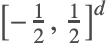 ,
 的一个完全对称积分规则由具有下述性质的的点的集合组成:(1) 一个集合中的所有点可以通过置换及/或改变集合中任意固定点坐标的符号生成;(2) 一个集合中的所有点都具有与之相关的相同权重.
NIntegrate[1 / Sqrt[x + y], {x, 0, 1}, {y, 0, 1}, Method -> "MultidimensionalRule"]满足上述性质的一个完全对称积分规则的点集被称为一个轨道. 轨道的一个点  ,若其坐标满足不等式
 ,则被称为一个生成元. (见 [KrUeb98][GenzMalik83].)
选项名称 | 默认值 | |
| "Generators" | 5 | 完全对称规则的生成元个数 |
| "SymbolicProcessing" | Automatic | 进行符号预处理需要的秒数 |
如果积分规则有  个分别记为
 的轨道,且其中的第
 个轨道
 的权重为
 ,则积分估计可通过下述公式进行计算:
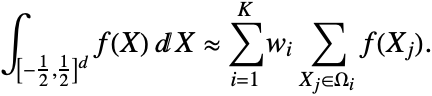
一个次数为  的空规则对于所有次数
 的单项式的积分为零,且对于对于至少一个次数为
 的单项式会失败. 每一个空规则可以被视作一个基本积分规则与一个次数较低的适当积分规则的差.
NIntegrate 的 "MultidimensionalRule" 对象基本上是三个积分对象的接口,将一个积分规则和一个或几个空规则合并. 下面的表格对生成元的个数和阶数作一总结. 具有6个和9个生成元的规则对象使用三个空规则,其中每一个是两个空规则的线性组合. 使用空规则的线性组合是为了防止相位误差. 关于如何使用空规则的更多细节请见[BerntEspGenz91].
| 生成元的个数 | 积分规则阶数 | 每一个空规则的阶 | 在何处被介绍 |
| 5 | 7 | 5 | [GenzMalik80] |
| 6 | 7 | 5,3,1 | [GenzMalik83][BerntEspGenz91] |
| 9 | 9 | 7,5,3 | [GenzMalik83][BerntEspGenz91] |


tbl = Table[Prepend[Table[
	(k = 0;NIntegrate[x ^ m + y ^ m, {x, 0, 1}, {y, 0, 1}, Method -> {"MultidimensionalRule", "Generators" -> gen}, EvaluationMonitor :> k++];k), {gen, {5, 6, 9}}], m], {m, 1, 20}];
Grid[Join[{{"单项式", "生成元个数", SpanFromLeft, SpanFromLeft}, {"degree", "5", "6", "9"}}, tbl], Dividers -> {{False, True, False}, {False, False, True, False}}, Alignment -> {Center}]
"MultidimensionalRule" 采样点和权重
numberOfGenerators = 9;MakeOrbit[generator_] :=
Module[{perms, signs, gperms, len = Length[generator]},
perms = Permutations[Range[len]];
signs = Flatten[Outer[List, Sequence@@Table[{1, -1}, {len}]], len - 1];
gperms = Map[Part[generator, #1]&, perms];
Union[Flatten[Outer[Times, gperms, signs, 1], 1]]
];dimension = 2;
precision = MachinePrecision;
rdata = NIntegrate`MultiDimensionalRuleData[numberOfGenerators, precision, dimension];
generators = rdata[[1, 1]];
weights = rdata[[1, 2]];orbits = MakeOrbit /@ generators;Clear[f]
f[x_, y_] := x ^ 3 * y ^ 3Total@MapThread[Total[Map[f@@(#1 + 1 / 2)&, #1] * #2]&, {orbits, weights}]//InputFormIntegrate[f[x, y], {x, 0, 1}, {y, 0, 1}]//N//InputFormgraphs = Graphics[{Red, AbsolutePointSize[4], Point /@ #1}, Axes -> False, AspectRatio -> 1, Frame -> True, FrameTicks -> None, PlotRange -> {{-1, 1}, {-1, 1}} / 2, ImageSize -> {75, 75}]& /@ orbits;Row[graphs]Graphics[First /@ graphs, Frame -> True, FrameTicks -> None]"LevinRule"
Levin 型规则通过用多项式和被积函数振荡部分的乘积对不定积分进行近似来估计振荡函数的积分.
NIntegrate[BesselJ[0, x + x^2], {x, 0, ∞}, Method -> "LevinRule"]默认时,"LevinRule" 自动检测被积函数的振荡部分,并应用下述配置方法来形成一个积分估计. 可以使用选项来指定振荡部分,并控制数值算法的细节行为,包括是否自适应地切换到一个备选的非振荡积分规则.
选项名称 | 默认值 | |
| "Points" | Automatic | 粗略的配置点数 |
| "EndpointLimitTerms" | Automatic | 在非数值端点的多项式外推阶 |
| "TimeConstraint" | 10 | 求解配置方程的最大时间 |
| "MethodSwitching" | True | 是否自动切换到非振荡规则 |
| "OscillationThreshold" | 10 | 应用 "LevinRule" 所需超过的近似振荡数 |
| Method | Automatic | 备选的非振荡规则 |
| "LevinFunctions" | Automatic | 包括在内核中的振荡函数 |
| "MaxOrder" | 50 | 内核的最大微分阶数 |
| ExcludedForms | {} | 被内核排除在外的形式 |
| "AdditiveTerm" | Automatic | 被积函数内附加的非振荡部分 |
| "Amplitude" | Automatic | 被积函数中内核的系数 |
| "DifferentialMatrix" | Automatic | 内核满足的线性常微分方程的矩阵形式 |
| "Kernel" | Automatic | 显式振荡内核 |
Levin 型配置方法
范围
一维数值积分的基本 Levin 型方法 [Levin96] 适用于如下形式的振荡积分:
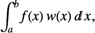
其中,振荡部分  必须满足阶数为
 的线性常微分方程(线性 ODE),以矩阵形式写作:
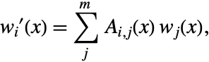
其中  是
 中的一个. 函数
 的向量是振荡“内核”,矩阵
 是“微分矩阵”.

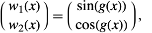

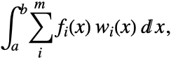
通常,上式比较简单的情况是  及
 . 函数
 的向量是“振幅”.
绝大多数振荡型特殊数学函数,如 Exp、BesselJ、AiryAi 等,满足线性常微分方程,因此可以利用 Levin 型方法进行积分. 此外,此类函数的任何乘积、求和或整数幂,或者是它们与任意非快速振荡函数的复合,仍满足线性常微分方程. 另请参见 DifferentialRootReduce.
"LevinRule" 方法可以应用于一种更一般的积分类别:
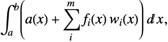
其中,“附加项”  通过一种传统的求积法,例如 "GaussKronrodRule",单独处理.
当振幅  、附加项
 以及微分矩阵
 自身非快速振荡时,Levin 型方法非常有效 [Levin97].
配置方法
在 Levin 型配置方法中,被积函数  的一个不定积分以
 的形式求出,其中
 是一些未知函数:

对等式两边关于  求导,并利用
 ,我们发现所有的
 可以消去,并且函数
 满足非振荡微分方程:
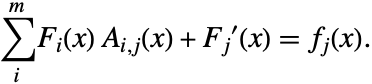
利用一种配置方法,这些方程中的  可以求解,在该配置方法中,我们将每个
 近似表示成一组
 个预定义的简单基函数
 的线性组合:
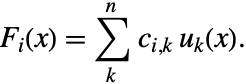
在 "LevinRule" 中,选取切比雪夫多项式 ChebyshevT[k,x] 作为基函数  . 将其代入关于
 的微分方程,得到
 个配置系数
 的
 个线性方程:

由于  、
 、
 和
 均为已知函数,我们可以在积分范围内部的
 个配置节点
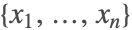 处计算这些线性方程. 这将生成关于
 个系数
 的
 个线性方程. 一旦得到这些方程的数值解,我们将得到
 的近似形式,并能够利用微积分基本定理来直接计算积分,如:

NIntegrate 使用与 "GaussKronrodRule" 对应的横坐标作为配置节点 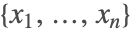 .
"LevinRule" 利用 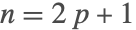 个配置节点计算积分估计,其中
 为 "Points" 方法选项的值. 同时,一个较低阶数的积分估计也利用每隔一点的配置节点 (
 ) 计算得到,这两个积分估计之差作为对算法误差的估计.
NIntegrate[Sin[x + x ^ 3], {x, 3, 1000}, Method -> {"LevinRule", "Points" -> 11}]指定振荡内核
默认时,"LevinRule" 自动选择构成被积函数尽可能多的部分作为振荡内核. 该行为可以通过选项进行细节修正.
如果被积函数包含的振荡函数在积分区域上不是高度振荡的,将其排除在振荡内核以外可能会更有效. 例如,Sin[x] 在区域 {x,0,5} 上不是高度振荡的.
NIntegrate[Sin[x]Sin[1000x], {x, 0, 5}, Method -> {"LevinRule", "Kernel" -> Sin[1000x]}]"ExcludedForms" 方法选项可用于指定不应包括在自动检测的振荡内核中的被积函数部分.
NIntegrate[Sin[x]Sin[1000x], {x, 0, 5}, Method -> {"LevinRule", ExcludedForms -> Sin[x]}]"LevinFunctions" 方法选项可用于指定哪种类型的函数可以包括在自动检测到的振荡内核中. 设置"LevinFunctions"->{h1,h2,…} 仅检测具体函数 hi.
NIntegrate[Sin[x]Exp[I x]BesselJ[0, x / 100], {x, 5, 500}, Method -> {"LevinRule", "LevinFunctions" -> {Exp, Sin}}]设置 "LevinFunctions"->{grp1,grp2,…} 检测已命名组 grpi 中的函数.
NIntegrate[Sin[x]Exp[I x]BesselJ[0, x / 100], {x, 5, 500}, Method -> {"LevinRule", "LevinFunctions" -> {"ExpRelated", "TrigRelated"}}]| "ExpRelated" | Exp、Power |
| "TrigRelated" | Sin、Cos、Sinh、Cosh、Haversine、Sinc |
| "ErfRelated" | Erf、Erfc、Erfi |
| "TrigIntegrals" | FresnelS、FresnelC、SinIntegral、CosIntegral, SinhIntegral、CoshIntegral |
| "BesselRelated" | BesselJ、BesselY、HankelH1、BesselI、BesselK, HankelH2、StruveH、StruveL、SphericalBesselJ |
| "AiryRelated" | AiryAi、AiryAiPrime、AiryBi、AiryBiPrime |
| "HypergeometricRelated" | HypergeometricPFQ、HypergeometricPFQRegularized, Hypergeometric0F1、Hypergeometric0F1Regularized, Hypergeometric2F1、Hypergeometric2F1Regularized |
| "InverseTrig" | ArcSin、ArcCos、ArcSinh、ArcCosh、ArcSec、ArcCsc、ArcSech、ArcCsch、ArcTan、ArcCot、ArcTanh、ArcCoth、InverseHaversine |
| "Elliptic" | EllipticE、EllipticK |
| "GammaRelated" | Gamma、GammaRegularized、Beta、BetaRegularized |
| "ExpIntegrals" | ExpIntegralE、ExpIntegralEi、DawsonF |
| "DifferentialRoots" | DifferentialRoot 对象 |
| "Other" | Log |
由 "LevinFunctions" 方法选项识别的已命名组.
缺省时,"LevinFunctions" 的设置除了包括 "Other"、"InverseTrig" 和 "Elliptic" 外,还包括所有已命名组. 该设置对应于定义域某些部分振荡的初等及特殊函数.
NIntegrate`LevinIntegrand 对象
利用内部函数 NIntegrate`LevinIntegrandReduce 对 NIntegrate 探测的振荡内核、微分矩阵、振幅与附加项进行详细检查是可能的. NIntegrate`LevinIntegrandReduce 返回一个 NIntegrate`LevinIntegrand 对象,该对象表示一个可以应用 Levin 型配置方法的完全处理的被积函数.
 +x

li = NIntegrate`LevinIntegrandReduce[x Exp[I x]BesselJ[0, 100x] + Sqrt[x], x]NIntegrate`LevinIntegrand 对象 li 的属性可以利用 li["prop"] 形式访问.

li["Kernel"]
First[li["DifferentialMatrices"]]//MatrixForm
D[li["Kernel"], x] == First[li["DifferentialMatrices"]].li["Kernel"]FullSimplify[%]li["Properties"]属性 "Rules" 给出用于 Levin 型配置算法的 NIntegrate`LevinIntegrand 的主要属性.


li["Rules"]利用该属性我们可以迅速查看不同 "LevinRule" 方法选项关于振荡内核检测的效果,例如 "AdditiveTerm" 选项.
NIntegrate`LevinIntegrandReduce[Sin[x] + Cos[x], x]["Rules"]NIntegrate`LevinIntegrandReduce[Sin[x] + Cos[x], x, "AdditiveTerm" -> Sin[x]]["Rules"]我们可以看到如何使用 "LevinFunctions" 选项将函数组包括在被积函数中或从被积函数中排除.
NIntegrate`LevinIntegrandReduce[Sin[x]Log[x], x, "LevinFunctions" -> Automatic]["Rules"]NIntegrate`LevinIntegrandReduce[Sin[x]Log[x], x, "LevinFunctions" -> All]["Rules"]完全指定被积函数分解的全部四部分(附加项、振幅、内核、微分矩阵)是可能的. 这可以用于对相似被积函数进行 NIntegrate 的有效多个调用.
NIntegrate[Sin[x] + Cos[x], {x, 5, 10}, Method -> {"LevinRule", "AdditiveTerm" -> Sin[x], "Amplitude" -> {1, 0}, "Kernel" -> {Cos[x], -Sin[x]}, "DifferentialMatrix" -> {{0, 1}, {-1, 0}}}]注意在这种情况下,NIntegrate 的第一个参数式完全被忽略了.
NIntegrate[ignored, {x, 5, 10}, Method -> {"LevinRule", "AdditiveTerm" -> Sin[x], "Amplitude" -> {1, 0}, "Kernel" -> {Cos[x], -Sin[x]}, "DifferentialMatrix" -> {{0, 1}, {-1, 0}}}]"MonteCarloRule"
蒙特卡洛规则通过形成一个在随机(半随机)采样点处被积函数值的统一加权和进行积分估计.
NIntegrate[(E^x - 1/E - 1), {x, 0, 1}, Method -> {"MonteCarloRule", "Points" -> 1000}]选项名称 | 默认值 | |
| "Points" | 100 | 采样点个数 |
| "PointGenerator" | Random | 采样点坐标生成器 |
| "AxisSelector" | Automatic | 全局自适应蒙特卡洛积分被使用时分裂轴的选择算法 |
| "SymbolicProcessing" | Automatic | 进行符号预处理需要的秒数 |
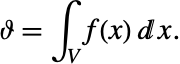
在 [KrUeb98] 的蒙特卡洛方法中, 维积分
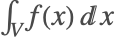 被解释成下述期望(平均)值:

其中  是函数
 相对于在
 上的均匀分布,被解释为一个随机变量时的平均值,即概率密度为
 的分布.
 代表区域
 上的特征函数;
 代表
 的体积.
期望值  的原始蒙特卡洛估计通过选取密度为
 的
 个独立随机向量
 得到(也就是说,向量在
 上均匀分布),并且得到估计
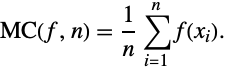
评注:函数  是一个有效的概率密度函数,因为它在整个
 上非负,并且
 .
根据强大数定律(strong law of large numbers),收敛

的概率为  . 强大数定律不提供关于误差
 的信息,因此使用一种概率估计.

公式 (3) 是  的无偏估计(即,对于
 的各种集合的期望值
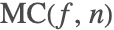 是
 )并且其方差是



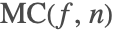


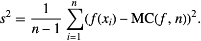
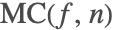


从方程 (4) 中可以看出,原始蒙特卡洛估计的收敛率不依赖于积分的维数  ,并且如果
 个采样点被使用,则收敛率为
 .
NIntegrate 的积分规则 "MonteCarloRule" 计算 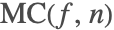 和
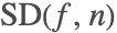 的估计值.
估计可以逐步得到改善. 也就是说,如果已知 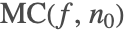 和
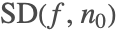 的估计和样本函数值
 的一个新的附加集合,则根据 (5) 和 (6),我们有


计算  和
 的估计时,没有必要知道计算
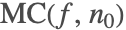 和
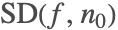 的估计所用的随机点.
"AxisSelector"
当用于多维全局自适应积分时,"MonteCarloRule" 采用两种方式选取一个积分子区域的分裂轴:(i) 随机选择,或 (ii) 如果子区域沿该轴被划分,则通过使每一半子区域的积分估计的方差和最小来选取. 分裂轴选取在积分估计之后进行.
通过下述方式进行轴的随机选择. "MonteCarloRule" 保留了供选择的轴的一个集合  . 初始情况下,
 包括所有的轴.
 的一个元素被随机选出. 选定的轴从
 中被排除. 在下一个积分估计之后,由
 中选择一个轴,并被排除在外,如此进行下去. 如果
 为空集,则被所有轴填充.
轴的最小方差选择通过下述方式完成. 在对该区域进行积分的过程中,采样点的一个子集及其被积函数值被存储. 然后对于每个轴,使用存储的采样点和相应的积分值来生成沿着这条轴线分开的两个子区域的方差. 使方差和最小的轴被选作分裂轴,因为这将意味着如果该区域被这个轴分开,则新的积分误差估计将最小. 如果对于某些轴,所有存储点集中于一个半区,则选用该轴进行区域的分割.
选项值 | |
| Random | 随机分裂轴选择 |
| MinVariance{MinVariance, "SubsampleFraction"->frac} | 分裂轴选择使新的区域的方差和最小的分裂轴选择 |
t = NIntegrate[Exp[-((x - 1 / 2)^2 + (y - 1 / 2)^2)], {x, 0, 1}, {y, 0, 1}, Method -> {"MonteCarloRule", "AxisSelector" -> Random}]在下面的的例子中,将两种选择轴的算法进行比较. 一般来说,使方差最小的选择使用的采样点较少,然而这种选法会使"MonteCarloRule" 的应用减慢. 因此,如果两种轴选择方法的使用导致相同的采样点数目,则使用随机轴选择方法较快. 此外,使用较大比例采样点,以选择使方差最小的分裂轴会导致积分速度的减慢.
f[x_ ? NumberQ, y_ ? NumberQ] := Boole[Abs[(x - (1/2))^2 + (y - (1/2))^2] < (1/6)] (E^-3 (x^2 + y^2) + (1/2));
Plot3D[f[x, y], {x, 0, 1}, {y, 0, 1}, PlotRange -> All, PlotPoints -> 20]t = Reap[NIntegrate[f[x, y], {x, 0, 1}, {y, 0, 1}, Method -> {"AdaptiveMonteCarlo", Method -> {"MonteCarloRule", "AxisSelector" -> Random}}, MinRecursion -> 1, PrecisionGoal -> 2.8, EvaluationMonitor :> Sow[{x, y}]]][[2, 1]];
Graphics[{PointSize[0.006], Point[t]}, AspectRatio -> 1, Frame -> True, PlotLabel -> "Number of sampling points = " <> ToString[Length[t]]]
t = Reap[NIntegrate[f[x, y], {x, 0, 1}, {y, 0, 1}, Method -> {"AdaptiveMonteCarlo", Method -> {"MonteCarloRule", "AxisSelector" -> {"MinVariance", "SubsampleFraction" -> 1 / 3}}}, MinRecursion -> 1, PrecisionGoal -> 2.8, EvaluationMonitor :> Sow[{x, y}]]][[2, 1]];Graphics[{PointSize[0.006], Point[t]}, AspectRatio -> 1, Frame -> True, PlotLabel -> "Number of sampling points = " <> ToString[Length[t]]]Do[NIntegrate[(1/Sqrt[x^2 + y^2]), {x, -1, 2}, {y, -1, 2}, Method -> {"AdaptiveMonteCarlo", Method -> {"MonteCarloRule", "Points" -> 500, "AxisSelector" -> Random}}], {100}]//TimingDo[NIntegrate[(1/Sqrt[x^2 + y^2]), {x, -1, 2}, {y, -1, 2}, Method -> {"AdaptiveMonteCarlo", Method -> {"MonteCarloRule", "Points" -> 500, "AxisSelector" -> {"MinVariance", "SubsampleFraction" -> 0.3}}}], {100}]//TimingDo[NIntegrate[(1/Sqrt[x^2 + y^2]), {x, -1, 2}, {y, -1, 2}, Method -> {"AdaptiveMonteCarlo", Method -> {"MonteCarloRule", "Points" -> 500, "AxisSelector" -> {"MinVariance", "SubsampleFraction" -> 0.6}}}], {100}]//Timing各种规则的比较
除了 "MonteCarloRule" 外,所有的规则都用于 NIntegrate 中的自适应策略. 一个积分策略的积分规则组件的类型及采样点的数目的更改是导致不同的积分算法. 一般来说,这些不同的积分算法在不同的积分中表现不同. 自然地会出现下述问题.
1. 对于某种类型的任意一个或几个积分,有没有一种类型的规则总是优于其它类型的规则?
2. 给定一种积分策略,哪一种规则的表现较好?是针对何种积分?
3. 已知一个积分,一种积分策略,以及一种积分规则,在这种规则下使用多少点能够在达到积分估计的目标且满足精确度的要求的前提下使采样点的总数最小?
对于一个给定的积分和积分策略,如果一种积分规则满足精确度要求,且采样点的数目最少,则称这种规则为最佳积分规则. 下面几个因素决定了最佳积分规则.
4. 一般来说,规则的次数越高,对于平滑的被积函数及较高的精确度目标,积分速度越快. 另一方面,规则次数有可能相对于被积函数而言过高而导致自适应策略在被积函数的不连续点处工作时的采样点过多.
5. 一个规则的误差估计函数显著影响积分策略的总工作量. 使用较少点的规则可能引起 (1) 由于对积分过低估计的错误结果,或者(2) 由于对积分过高估计而使用过多的采样点. (见 "病态行为范例".) 此外,误差估计函数可能采用一个或几个嵌入的空规则进行计算. 一般来说,空规则的数量越多,误差估计的效果越好—因为相位误差越少. 空规则的数量和及其在计算误差估计的加权和中被指定的权重决定了病态积分和难以用该规则进行计算的积分的集合. (NIntegrate 中的一些多维规则使用嵌入的空规则进行误差估计的计算. NIntegrate 中的所有一维积分规则都只使用一种空规则.)
6. 局部自适应策略对于采样点趋于均匀分布的的封闭规则(例如 "ClenshawCurtisRule") 比开放规则(例如GaussKronrodRule)和采样点非均匀分布的的封闭规则(例如 "LobattoKronrodRule")更为有效.
7. 被策略重复使用的点的百分比可在很大程度上决定哪一种规则最好. 对于一维积分,"LocalAdaptive" 重复使用封闭规则的所有点. "GlobalAdaptive" 则放弃误差估计有待改善的区域的几乎所有点.
一个规则中点的数目
这一小节用实例说明规则的次数越高,对于平滑的被积函数及较高的精确度目标,积分速度越快. 同时也用例子说明规则次数相对于被积函数过高而导致自适应策略在被积函数的不连续点处工作时使用的采样点过多. 这些例子均使用高斯规则及 Berntsen–Espelid误差估计.


(见 [DavRab84].)

RuleError[f_, rule_String, prec_, pnts_ ? NumberQ] :=
	Block[{absc, weights, errweights},
	{absc, weights, errweights} = ToExpression["NIntegrate`" <> rule <> "Data"][pnts, prec];
	Abs[Total[MapThread[f[#1]#2&, {absc, weights}]] - Integrate[f[x], {x, 0, 1}]]
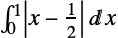
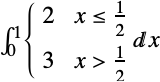
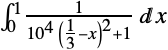
];funcs = {Sqrt[x], Abs[x - (1/E)], | | |
| :- | :-------- |
| 2 | x ≤ (1/E) |
| 3 | x > (1/E) |, (1/10^4 ((1/π) - x)^2 + 1)};
Row[Plot[#, {x, 0, 1}, PlotRange -> All, Frame -> True, FrameTicks -> {None, Automatic}, ImageSize -> {120, 120}]& /@ funcs, " "]
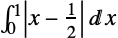
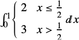
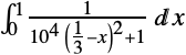
errors = Table[{pnts, RuleError[#, "GaussBerntsenEspelidRule", 30, pnts]}, {pnts, 4, 100, 1}]& /@ Function /@ (Function[{f}, f /. x -> #] /@ funcs);gr = ListLinePlot[MapThread[Tooltip[{#[[1]], Log[10, #[[2]]]}& /@ #1, #2]&, {errors, funcs}], PlotRange -> {{0, 100}, {0, -9}}, AxesOrigin -> {0, 0}, ImageSize -> {300}];
xc = 110;
xcSq = 106;
legend = {Text[funcs[[1]], {xc, -2}, {-1, 0}], Text[funcs[[2]], {xc, -4}, {-1, 0}], Text[funcs[[3]], {xc, -6}, {-1, 0}], Text[funcs[[4]], {xc, -8}, {-1, 0}]};
legendSq = {Text[" ", {xcSq, -2}, {-1, 0}], Text[" ", {xcSq, -4}, {-1, 0}], Text[" ", {xcSq, -6}, {-1, 0}], Text[" ", {xcSq, -8}, {-1, 0}]};
legendSq = MapThread[Append[#1, Background -> #2]&, {legendSq, Cases[gr, Hue[s__], ∞]}];
Row[{gr, " ", Graphics[{ legend, legendSq}, ImageSize -> {200, 200}, AspectRatio -> 5]}]采样点的最小数目
Attributes[SamplingPoints] = {HoldFirst};
SamplingPoints[expr_] :=
	Module[{k = 0, res},
res = Hold[expr] /. HoldPattern[NIntegrate[s___]] :> NIntegrate[s, EvaluationMonitor :> k++];ReleaseHold[res];k]tblga = Table[{pg, pnts, SamplingPoints[NIntegrate[#, {x, 0, 1}, Method -> {"GlobalAdaptive", "SymbolicProcessing" -> 0, Method -> {"GaussBerntsenEspelidRule", "Points" -> pnts}}, MaxRecursion -> 100, WorkingPrecision -> 35, PrecisionGoal -> pg]]}, {pg, 4, 30}, {pnts, 4, 25}]& /@ funcs;minPnts = (#[[Position[#, Min[#[[3]]& /@ #]][[1, 1]]]]&[#]& /@ #)& /@ tblga;gr = ListLinePlot[(Drop[#, -1]& /@ #)& /@ minPnts, PlotRange -> {{0, 30}, {0, 26}}, PlotStyle -> Thickness[0.003], AxesOrigin -> {3, 0}, ImageSize -> {300, 200}];
xc = 110;
xcSq = 106;
legend = {Text[funcs[[1]], {xc, -2}, {-1, 0}], Text[funcs[[2]], {xc, -4}, {-1, 0}], Text[funcs[[3]], {xc, -6}, {-1, 0}], Text[funcs[[4]], {xc, -8}, {-1, 0}]};
legendSq = {Text[" ", {xcSq, -2}, {-1, 0}], Text[" ", {xcSq, -4}, {-1, 0}], Text[" ", {xcSq, -6}, {-1, 0}], Text[" ", {xcSq, -8}, {-1, 0}]};
legendSq = MapThread[Append[#1, Background -> #2]&, {legendSq, Cases[gr, Hue[s__], ∞]}];
Row[{gr, " ", Graphics[{ legend, legendSq}, ImageSize -> {200, 200}, AspectRatio -> 5]}]规则比较

RuleErrors[f_, rule_String, prec_, pnts_ ? NumberQ] :=
	Block[{absc, weights, errweights},
	{absc, weights, errweights} = ToExpression["NIntegrate`" <> rule <> "Data"][pnts, prec];
	{Abs[Total[MapThread[f[#1]#2&, {absc, weights}]] - Integrate[f[x], {x, 0, 1}]], Abs[Total[MapThread[f[#1]#2&, {absc, errweights}]]]}
];funcs = {Sqrt[x], Abs[x - (1/E)], | | |
| :- | :-------- |
| 2 | x ≤ (1/E) |
| 3 | x > (1/E) |, (1/10^4 ((1/π) - x)^2 + 1)};
Row[Plot[#, {x, 0, 1}, PlotRange -> All, Frame -> True, FrameTicks -> {None, Automatic}, ImageSize -> {120, 120}]& /@ funcs, " "] ,
 ,
 和
 中的每个积分使用"GaussKronrodRule", "LobattoKronrodRule", "TrapezoidalRule" 和"ClenshawCurtisRule" 的误差:
rules = {"GaussKronrodRule", "LobattoKronrodRule", "TrapezoidalRule", "ClenshawCurtisRule"};
errors = Outer[Table[{pnts, RuleErrors[#2, #1, 30, pnts]}, {pnts, 4, 100, 1}]&, rules, Function /@ (Function[{f}, f /. x -> #] /@ funcs)];
exactErrors = Map[#[[1]]&, errors, {-2}];
ruleErrors = Map[#[[2]]&, errors, {-2}];Row[{Grid[Join[{{"exact errors", "error estimates"}}, Flatten[Transpose[{{#, SpanFromLeft}& /@ rules, Transpose[Map[
Function[{d},
(gr = ListLinePlot[Map[{#[[1]], Log[10, #[[2]]]}& /@ #&, d], ImageSize -> {200, 100}, PlotRange -> {{0, 100}, {0, -9}}, AxesOrigin -> {0, 0}];
xc = 110;
xcSq = 106;
legend = {Text[funcs[[1]], {xc, -1.5}, {-1, 0}], Text[funcs[[2]], {xc, -3.5}, {-1, 0}], Text[funcs[[3]], {xc, -5.5}, {-1, 0}], Text[funcs[[4]], {xc, -7.5}, {-1, 0}]};
legendSq = {Text[" ", {xcSq, -1.5}, {-1, 0}], Text[" ", {xcSq, -3.5}, {-1, 0}], Text[" ", {xcSq, -5.5}, {-1, 0}], Text[" ", {xcSq, -7.5}, {-1, 0}]};
legendSq = MapThread[Append[#1, Background -> #2]&, {legendSq, Cases[gr, Hue[s__], ∞]}];
gr)], {exactErrors, ruleErrors}, {2}]]}], 1]], Dividers -> All], Graphics[{legend, legendSq}, ImageSize -> {200, 200}, AspectRatio -> 5]}]病态行为范例
针对误差估计的错误行为
这一小节将讨论这样一种积分:NIntegrate 在默认设置下由于不能检测被积函数的一部分而对积分估计不足. 如果精确度目标提高则这一部分将被检测到.
错误估计
f[x_] := Sech[10 * (x - 0.2)] ^ 2 + Sech[100 * (x - 0.4)] ^ 4 + Sech[1000 * (x - 0.6)] ^ 6
exact = Integrate[f[x], {x, 0, 1}]est = NIntegrate[f[x], {x, 0, 1}]Abs[exact - est]Plot[f[x], {x, 0, 1}]较好的结果
NIntegrate[f[x], {x, 0, 1}, Method -> "GlobalAdaptive", MaxRecursion -> 20, PrecisionGoal -> 12]
Table[{pg, NIntegrate[f[x], {x, 0, 1}, Method -> "GlobalAdaptive", MaxRecursion -> 20, PrecisionGoal -> pg]}, {pg, 6, 12}]



Plot[f[x], {x, 0, 1}, PlotPoints -> 100]eps = 0.0015;Plot[f[x], {x, 0.6 - eps, 0.6 + eps}]NIntegrate[f[x], {x, 0.6 - eps, 0.6 + eps}]Abs[exact - est]为什么估计受到误导
{absc, weights, errweights} = NIntegrate`GaussKronrodRuleData[5, MachinePrecision];IRuleEstimate[f_, {a_, b_}] :=
Module[{integral, error},
{integral, error} = (b - a)Total@MapThread[{f[#1]#2, f[#1]#3}&, {Rescale[absc, {0, 1}, {a, b}], weights, errweights}];
{integral, Abs[error]}
]cTbl = Reap[NIntegrate[f[x], {x, 0, 1},
EvaluationMonitor :> Sow[x]]][[2]]//Flatten;ListPlot[Transpose[{cTbl, Range[1, Length[cTbl]]}], AspectRatio -> 0.5, PlotRange -> {{0, 1}, {0, Length[cTbl]}}, PlotStyle -> {Hue[0.7]}]可以看出在前面的图形中 NIntegrate 在靠近  的第二个尖峰处进行大量计算. NIntegrate 不在靠近
 的不积分的峰处进行同样量的计算.
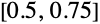
gk = Sort[Take[cTbl, -11]]
g = Take[gk, {2, -2, 2}]fgk = f /@ gk;
fg = f /@ g;gkf[x_] := Evaluate[InterpolatingPolynomial[Transpose[{gk, fgk}], x]]
gf[x_] := Evaluate[InterpolatingPolynomial[Transpose[{g, fg}], x]]
Plot[{gkf[x], gf[x]}, {x, Min[gk], Max[gk]}]
eps = 0.01;
Plot[{gkf[x], gf[x]}, {x, 0.6 - eps, 0.6 + eps}]
Integrate[gkf[x], {x, 0.5, 0.75}]
Integrate[gf[x], {x, 0.5, 0.75}]
% - %%//FullForm
由于这个差值就是区域 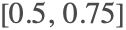 所指定的误差估计,在默认的精确度目标下,NIntegrate 不会用它进行进一步的积分完善.
相位误差
这一小节将讨论导致积分规则对积分估计的实际误差严重过高或过低估计的原因. 在 [LynKag76] 中给出了类似的讨论.
f[x_, λ_, μ_] := (10^-μ/(x - λ)^2 + 10^-2μ)
num = NIntegrate[f[x, 0.415, 1.25], {x, -1, 1}, PrecisionGoal -> 2]exact = Integrate[f[x, 0.415, 1.25], {x, -1, 1}]
Abs[num - exact] / Abs[exact](注意对于较高的精确度目标,NIntegrate 给出正确结果.)
令积分规则  嵌入到规则
 中. 偶尔,积分估计
 (其中
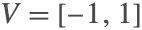 )的误差估计
 与准确误差
 相比可能过小.


{absc, weights, errweights} = NIntegrate`GaussKronrodRuleData[5, MachinePrecision];IRuleEstimate[f_, {a_, b_}] :=
Module[{integral, error},
{integral, error} = (b - a)Total@MapThread[{f[#1]#2, f[#1]#3}&, {Rescale[absc, {0, 1}, {a, b}], weights, errweights}];
{integral, Abs[error]}
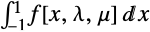
]
exact = -ArcTan[10^μ (-1 + λ)] + ArcTan[10^μ (1 + λ)];




Block[{λ, μ = 1.15, pnts = 1000, rres, errres, exactres, lambdas},
	(* the plot uses 1000 values λ *)
	lambdas = Table[λ, {λ, -1, 1, (2/pnts - 1)}];
	(* this computes the integral and error esitmates over the λ's *)
	{rres, errres} = Transpose@Map[Function[{λ}, IRuleEstimate[f[#1, λ, Evaluate[μ]]&, {-1, 1}]], lambdas];

	(* this computes the exact integrals over the λ's *)
	exactres  = Map[exact /. λ -> #1&, lambdas];

	(* this finds the number underestimating error estimates *)
	Print["Percent of underestimation: ", 100 * Length[Select[errres - Abs[exactres - rres], #1 < 0&]] / Length[lambdas]//N, "%", " "];

	(* the plots, blue is for  | GK[f, 5] - GK[f, 5] | , red is for  | GK[f, 5] - Subsuperscript[∫, -1, 1]f[x, λ, μ] |  *)
	ListLinePlot[{Transpose[{lambdas, errres}], Transpose[{lambdas, Abs[exactres - rres]}]}, PlotRange -> All, PlotStyle -> {{Hue[0.7]}, {Hue[0]}}, AxesLabel -> {λ, "error"}]
	]
在上面的图形中,蓝色图线代表估计的误差  . 实际误差
 的图线为红色.
可以看到,参数  的值 0.415 非常接近于
 的一个局部最小值.
一个一维求积法规则可以看作一个根据规则的横坐标及其对应的被积函数值拟和的多项式的积分结果. 我们可以进一步尝试看到 f[x,λ,μ] 的积分的拟合多项式.
Clear[FitPlots];
FitPlots[f_, {a_, b_}, abscArg_] :=
	Module[{absc = Rescale[abscArg, {0, 1}, {a, b}]},
	(* this finds the interpolating polynomial through the Gauss abscissas and the values of f over them *)
	polyGauss[x_] := Evaluate[InterpolatingPolynomial[Transpose[{Take[absc, {2, -2, 2}], f[#1]& /@ (Take[absc, {2, -2, 2}])}], x]];

	(* this finds the interpolating polynomial through the Gauss-Kronrod abscissas and the values of f over them *)
	polyGaussKronrod[x_] := Evaluate[InterpolatingPolynomial[Transpose[{absc, f[#1]& /@ absc}], x]];

	(* plot of the Gauss interpolating points *)
	samplPointsGauss = Graphics[{GrayLevel[0], PointSize[0.02], Point /@ Transpose[{Take[absc, {2, -2, 2}], f[#1]& /@ Take[absc, {2, -2, 2}]}]}];

	(* plot of the Gauss-Kronrod interpolating points *)
	samplPointsGaussKronrod = Graphics[{Red, PointSize[0.012], Point /@ Transpose[{absc, f[#1]& /@ absc}]}];

	(* interpolating polynomials and f plots *)
	Block[{$DisplayFunction = Identity},
	funcPlots = Plot[{polyGauss[x], polyGaussKronrod[x], f[x]}, {x, a, b}, PlotRange -> All, PlotStyle -> {{Hue[0.7]}, {Hue[0.8]}, {Hue[0]}}];
	];

	exact = Integrate[f[x], {x, a, b}];
	r1 = Integrate[polyGauss[x], {x, a, b}];
	r2 = Integrate[polyGaussKronrod[x], {x, a, b}];
	Print["estimated integral:" <> ToString@r2, "  exact integral:" <> ToString@Re@exact];
	Print["estimated error:" <> ToString@Abs[r1 - r2], "  actual error:" <> ToString@Abs[r2 - exact]];
	Show[{funcPlots, samplPointsGauss, samplPointsGaussKronrod}]
	];
下面的图形中,函数 f[x,λ,μ] 为红色,高斯多项式为蓝色,高斯–Kronrod 多项式为紫色,高斯采样点为黑色,高斯–Kronrod 采样点为红色.
可以看到由于 f[x,0.415,1.25] 的峰值大致落到两个横坐标的中间,这一近似为过低估计.
FitPlots[f[#1, 0.415, 1.25]&, {-1, 1}, absc]

相反地,由于 f[x,0.53,1.25] 的峰值大致落到一个横坐标上,该近似为过高估计.
FitPlots[f[#1, 0.53, 1.25]&, {-1, 1}, absc]
