EmptySpaceF[pdata,r]
半径 r にある点データ pdata について空空間関数  を推定する.
EmptySpaceF[pproc,r]
点データ pproc について  を計算する.
EmptySpaceF[bdata,r]
ビン分割データ bdata について  を計算する.
EmptySpaceF[pspec]
異なる半径 r に繰り返し適用可能な関数  を生成する
を生成する

EmptySpaceF
EmptySpaceF[pdata,r]
半径 r にある点データ pdata について空空間関数  を推定する.
EmptySpaceF[pproc,r]
点データ pproc について  を計算する.
EmptySpaceF[bdata,r]
ビン分割データ bdata について  を計算する.
EmptySpaceF[pspec]
異なる半径 r に繰り返し適用可能な関数  を生成する
を生成する
詳細とオプション
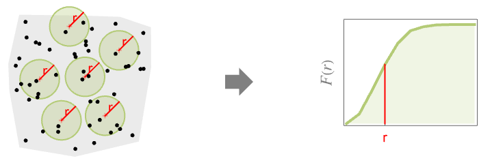
- EmptySpaceFは,球状接触分布関数としても知られている.
- 関数
 は,通常 pdata の点ではない任意の場所から距離
  内にある点を求める確率を与える.
 -
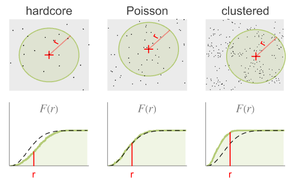
- ポアソン(Poisson)点過程と比較すると,結果は以下のようになる.
-
- 半径 r は単一の値でも値のリストでもよい.半径 r が指定されていないと,EmptySpaceFは
 関数を繰り返し評価するために使えるPointStatisticFunctionを返す.
 - 点データ pdata の形式は以下の形でよい.
-
{p1,p2,…} 点 pi GeoPosition[…],GeoPositionXYZ[…],… 地理的点 SpatialPointData[…] 空間点集合 {pts,reg} 点集合 pts と観測領域 reg - 観測領域 reg は,与えられていなければRipleyRassonRegionを使って自動的に計算される.
- 点過程 pproc は次の形でよい.
-
proc 点過程 proc {proc,reg} 点過程 proc と観測領域 reg - 観測領域 reg は,パラメータフリーのSpatialObservationRegionQでなければならない.
- ビン分割データ bdata はSpatialBinnedPointDataからのもので,区分一定強度関数によってInhomogeneousPoissonPointProcessとして扱われる.
- pdata について,
 は観測領域を離散化することで計算され,一定の点強度が想定される.
 - pproc について,
 は厳密な式を使うことで,あるいはシミュレーションで点データを生成することで計算される.
 - 次は,使用可能なオプションである.
-
Method Automatic 使用するメソッド SpatialBoundaryCorrection Automatic 使用する境界補正 - 次は,SpatialBoundaryCorrectionの可能な設定である.
-
Automatic 境界補正を自動的に決定する None 境界補正なし "BorderMargin" 観測領域に内部余白を使う "Hanisch" 最近傍までの距離が境界までの距離より大きい点を削除する "KaplanMeier" SurvivalDistributionメソッド.点の最近傍までの距離が領域境界までの距離で打ち切られる "NelsonAalen" SurvivalDistributionメソッド.点の最近傍までの距離が領域境界までの距離で打ち切られる - Method->{"Discretization"->opts}と設定することで推定における離散かメソッドが調整できる.opts はDiscretizeRegionの任意の有効なオプションでよい.
例題
すべて開く すべて閉じる例 (3)
region = Ball[{0, 0}];
pts = RandomPoint[region, 100];EmptySpaceF[{pts, region}, 0.1]spd = SpatialPointData[RandomReal[1, {100, 2}]]rspec = Range[0.01, 0.2, 0.01];est = EmptySpaceF[spd, rspec];ListPlotで結果を可視化する:
ListPlot[est, DataRange -> MinMax[rspec], Filling -> Axis, AxesLabel -> {r}]f = EmptySpaceF[ThomasPointProcess[3, 2, 0.2, 2], r];Plot[f, {r, 0, 0.5}, AxesLabel -> Automatic]スコープ (7)
点データ (4)
region = Rectangle[{0, 0}, {1, 2}];
pts = RandomPoint[region, 100];EmptySpaceF[{pts, region}, 0.1]指定された距離のリストについての空空間関数の経験的推定値を得る:
EmptySpaceF[{pts, region}, {0.1, 0.15, 0.01, 0.03}]後で使えるようにPointStatisticFunctionを作る:
reg = Disk[];
pts = RandomPoint[Disk[], 100];psf = EmptySpaceF[{pts, reg}]psf[0.1]BlockRandom[SeedRandom[1];
pts = RandomReal[1, {100, 2}]
];psf = EmptySpaceF[pts]psf["ObservationRegion"]
psf[0.05]EmptySpaceFをGeoPositionと一緒に使う:
pts = RandomGeoPosition[GeoDisk[GeoPosition[{0, 0}], Quantity[10, "Kilometers"]], 10 ^ 2]psf = EmptySpaceF[pts]ListPlot[Table[{x, psf[x]}, {x, Quantity[0, "km"], psf["MaxRadius"], Quantity[.1, "km"]}], AxesLabel -> {"km"}]点過程 (3)
PoissonPointProcessについての空空間関数は閉じた形を持つ:
proc = PoissonPointProcess[μ, d];EmptySpaceF[proc, r]Plot[Table[EmptySpaceF[proc /. μ -> 2, r], {d, 1, 4}]//Evaluate, {r, 0, 1.3}, AxesLabel -> {r}, PlotLegends -> (Row[{#, "D"}]& /@ Range[4])]指定次元のクラスタ過程ThomasPointProcessについての空空間関数:
proc2D = ThomasPointProcess[30, 10, .3, 2];DiscretePlot[EmptySpaceF[proc2D, r], {r, 0.01, .5, .02}, PlotRange -> {0, 1}, AxesLabel -> Automatic]proc3D = ThomasPointProcess[30, 10, .3, 3];DiscretePlot[EmptySpaceF[proc3D, r], {r, 0.01, .5, .02}, PlotRange -> {0, 1}, AxesLabel -> Automatic]指定次元のクラスタ過程MaternPointProcessについての空空間関数:
proc2D = MaternPointProcess[30, 5, 1, 2];DiscretePlot[EmptySpaceF[proc2D, r], {r, 0.01, .5, .02}, PlotRange -> {0, 1}, AxesLabel -> Automatic]proc3D = MaternPointProcess[30, 5, 1, 3];DiscretePlot[EmptySpaceF[proc3D, r], {r, 0.01, .5, .02}, PlotRange -> {0, 1}, AxesLabel -> Automatic]オプション (3)
SpatialBoundaryCorrection (2)
境界補正なしのEmptySpaceF推定器は偏っているので,大きい点集合以外では使うべきではない:
region = Rectangle[{0, 0}, {1, 2}];
pts = RandomPoint[region, 100];EmptySpaceF[{pts, region}, 0.1, SpatialBoundaryCorrection -> "None"]デフォルトメソッドの"BorderMargin"は境界から距離  の点だけを考慮する:
EmptySpaceF[{pts, region}, 0.1, SpatialBoundaryCorrection -> "BorderMargin"]"Hanisch"法は観測領域の各点に重みを付けて,推定値が偏らないようにする:
EmptySpaceF[{pts, region}, 0.1, SpatialBoundaryCorrection -> "Hanisch"]"KaplanMeier"法と"NelsonAalen"法はSurvivalDistributionで使われる推定器である.各点から最近傍までの距離は各点から観測領域の境界までの距離で打ち切られる:
EmptySpaceF[{pts, region}, 0.1, SpatialBoundaryCorrection -> "KaplanMeier"]EmptySpaceF[{pts, region}, 0.1, SpatialBoundaryCorrection -> "NelsonAalen"]region = Disk[];
pts = RandomPoint[region, 400];rlist = Range[0.01, 0.1, 0.005];
mths = {"BorderMargin", "Hanisch", "KaplanMeier"};data = EmptySpaceF[{pts, region}, rlist, SpatialBoundaryCorrection -> #]& /@ mths;f[r_] := 1 - Exp[-(400 / RegionMeasure[region])(Pi)r ^ 2]Show[Plot[f[r], {r, 0, 0.1}, PlotStyle -> Gray, PlotLegends -> {"theoretical"}], ListPlot[data, DataRange -> MinMax[rlist], PlotLegends -> mths], AxesLabel -> {r}]Method (1)
離散か設定はMethodのサブオプションとして与えることができる:
region = Triangle[{{0, 0}, {1, 2}, {-3, 1}}];
pts = RandomPoint[region, 100];同じ半径の空空間をMaxCellMeasureの値を変えて推定する:
EmptySpaceF[{pts, region}, 0.05, Method -> {"Discretization" -> {MaxCellMeasure -> #}}]& /@ {0.005, 0.01, 0.02}異なる離散化メソッドを使って同じ半径における空空間関数を推定する:
EmptySpaceF[{pts, region}, 0.05, Method -> {"Discretization" -> {Method -> #}}]& /@ {"Continuation", "DiscretizeGraphics"}アプリケーション (3)
data1 = RandomPointConfiguration[PoissonPointProcess[20, 2], Disk[]];
data2 = RandomPointConfiguration[InhomogeneousPoissonPointProcess[Function[{x, y}, (20x ^ 2 + 40y ^ 2)], 2], Disk[]];F1 = EmptySpaceF[data1];
F2 = EmptySpaceF[data2];Plot[{F1[r], F2[r]}, {r, 0, 1}, PlotRange -> All, AxesLabel -> {r}]rr = {0.05, 0.1, 0.15};
spds = Table[RandomPointConfiguration[HardcorePointProcess[100, rad, 2], Disk[]], {rad, rr}];Fs = Table[EmptySpaceF[spd], {spd, spds}];DiscretePlot[Map[#[r]&, Fs]//Evaluate, {r, 0.005, 0.2, 0.005}, AxesLabel -> {r}, PlotLegends -> (Row[{"rad = ", #}]& /@ rr)]2019年5月20日(月)に,暴風予報センターが,テキサス州のパンハンドルの北東部からオクラホマ州中央部までの小さな回廊を指摘した.EF2–EF5竜巻が特定の場所から25マイル以内で発生する確率は45%で,これがEmptySpaceFの値を定義する:
eqn[proc_] := (EmptySpaceF[proc, Quantity[25, "Miles"]] == .45)領域上の強度が一定であると仮定して,ポアソン点過程を竜巻のパターンモデルとして使う:
eqn[PoissonPointProcess[λ, 2]]sol = First@Solve[eqn[PoissonPointProcess[λ, 2]], λ]
model = PoissonPointProcess[λ /. sol, 2]Plot[EmptySpaceF[model, Quantity[r, "Miles"]], {r, 0, 50}, AxesLabel -> {"Miles"}]オクラホマ州上の可能な竜巻の広がりのシミュレーションを行う:
OK = RandomPointConfiguration[model, Entity["AdministrativeDivision", {"Oklahoma", "UnitedStates"}]["Polygon"]]GeoListPlot[OK["Points"], GeoRange -> Entity["AdministrativeDivision", {"Oklahoma", "UnitedStates"}]]特性と関係 (4)
空空間関数はCDFのように動作する:
data = RandomPointConfiguration[PoissonPointProcess[20, 2], Disk[]];F = EmptySpaceF[data]Plot[F[r], {r, 0, 1}, PlotRange -> All]PoissonPointProcessについての空空間関数は,半径  の円板上のPointCountDistributionの零点におけるSurvivalFunctionに等しい:
proc[d_] := PoissonPointProcess[μ, d]EmptySpaceF[proc[d], r]
dist[d_] := PointCountDistribution[proc[d], Ball[ConstantArray[0, d], r]];SurvivalFunction[dist[2], 0] === EmptySpaceF[proc[2], r]SurvivalFunction[dist[3], 0] === EmptySpaceF[proc[3], r]With[{d = RandomInteger[10 ^ 6]}, SurvivalFunction[dist[d], 0] === EmptySpaceF[proc[d], r]]PoissonPointProcessの空空間関数と最近傍関数は等しい:
proc = PoissonPointProcess[μ, d];EmptySpaceF[proc, r]NearestNeighborG[proc, r]%% - %1Dでは,両者はどちらもExponentialDistributionの累積分布関数に等しい:
vol[d_] := π ^ (d / 2) / Gamma[1 + d / 2]CDF[ExponentialDistribution[μ * vol[1]], r]Block[{d = 1}, % == EmptySpaceF[proc, r] == NearestNeighborG[proc, r]//Simplify[#, r ≥ 0]&]EmptySpaceFはしばしばNearestNeighborGと比較されるが,後者は点集合内の点から距離 r 内に別の点が見付かる確率を推定するものである:
region = Ball[{0, 0}];
pts = RandomPoint[region, 1000];rspec = Range[0, 0.08, 0.005];
res = NearestNeighborG[{pts, region}, rspec];結果をListPlotで可視化する:
ListPlot[res, DataRange -> MinMax[rspec], Filling -> Axis, AxesLabel -> {r}]HardcorePointProcessが生成した点データについてのEmptySpaceFとNearestNeighborGの推定を比較する:
spd1 = RandomPointConfiguration[HardcorePointProcess[500, 0.15, 2], region]rspec1 = Range[0, 0.3, 0.01];
esf = EmptySpaceF[spd1, rspec1];
nng = NearestNeighborG[spd1, rspec1];ListLinePlot[{nng, esf}, DataRange -> MinMax[rspec1], Filling -> Axis, AxesLabel -> {r}, PlotLegends -> {"Nearest Neighbor Distribution", "Empty Space Distribution"}]テキスト
Wolfram Research (2020), EmptySpaceF, Wolfram言語関数, https://reference.wolfram.com/language/ref/EmptySpaceF.html.
CMS
Wolfram Language. 2020. "EmptySpaceF." Wolfram Language & System Documentation Center. Wolfram Research. https://reference.wolfram.com/language/ref/EmptySpaceF.html.
APA
Wolfram Language. (2020). EmptySpaceF. Wolfram Language & System Documentation Center. Retrieved from https://reference.wolfram.com/language/ref/EmptySpaceF.html