Line
詳細とオプション
- Lineは,ポリラインあるいは線分としても知られている.
- Lineは,幾何学領域として,またグラフィックスプリミティブとして使うことができる.
- Lineは,piから pi+1までの線分が
 で与えられる,区間ごとの線形曲線を表す.
 - Lineは,GraphicsおよびGraphics3Dで使うことができる.
- グラフィックスでは,点 piは,Scaled,Offset,ImageScaled,Dynamicの各式でよい.
- グラフィックスの描画は,Thickness,Dashing,JoinForm,CapForm,色等の指示子の影響を受ける.
- グラフィックスで使用可能なオプションと設定値
-
VertexColors None 補間される頂点の色 VertexNormals None 陰影付けのための有効な頂点の法線 - Lineは,GeometricSceneの記号の点と一緒に使うことができる.
予備知識
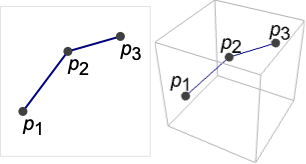
- Lineは,幾何学的な線分あるいは連結された一連の線分(ポリライン)を表すグラフィックスおよび幾何学上のプリミティブである.
 次元空間において
  個の点を繋ぐLineの位置は,
 個のサブリストからなる引数のリストとして指定することができる.各サブリストには
  個の直交座標の値が含まれる.Lineオブジェクトの座標サブリストは,厳密値あるいは近似値からなる.ここで,RegionEmbeddingDimensionを使って,与えられたLine式についての次元
  を特定することができる.線の集合(ポリライン)は,単一のLineプリミティブ(マルチライン)内の
  個のタプルのネストしたリストとして表すことができる.Lineオブジェクトの座標は厳密値でも近似値でもよい.
 - GraphicsおよびGraphics3Dを使って,Lineオブジェクトを二次元あるいは三次元で視覚的にフォーマットすることができる.Lineオブジェクトは,GeoGraphicsおよびGeoPositionを使って地理学的な地図で使うこともできる(例:GeoGraphics[Line[GeoPosition[{{38.9,-77.0},{40.1,-88.3}}]]]).Lineは計算が行われる領域の指定としても使うことができる.
- 線自体の次元は(RegionDimension関数によって表される通り)1であり,太さはゼロであるが,フォーマットされたグラフィックス式中のLineオブジェクトは,デフォルトで,一次元の数学的線よりも太く見えるようにスタイル付けされる.さらに,グラフィカルな可視化においては,視点からの距離による大きさの違いとは無関係に,線は同じ大きさで表示される.グラフィックスにおけるLineオブジェクトの外観は,Thickness,AbsoluteThickness,Thick,Thin等の太さの指示子,Dashing,AbsoluteDashing,Dashed,Dotted,DotDashed等の破線指示子,EdgeForm,CapForm等の辺とキャップの指示子,Red等の色指示子,透過性指示子Opacity,スタイルオプションAntialiasingを指定することで変更できる.また,複数の線の色はVertexColorsを使って指定することができ,Graphics3D内の複数の線の陰影付けやシミュレーションによる照明はVertexNormalsを使って指定することができる.
- GeometricTransformationや,より明確な変換関数のTranslateおよびRotateを使って,もとになっているLine式を変更せずにLineオブジェクトが表示される座標を変えることができる.
- Tube,Arrow,HalfLine,InfiniteLine等の他のグラフィックスプリミティブは,スタイル付けされたLineオブジェクトのグラフィックスプリミティブに似ていることがある.ポリラインはまっすぐな線分のみからなるが,BSplineCurveあるいはBezierCurveを使ってスプラインから,あるいはInterpolationを使って補間関数から,曲線を構築することができる.幾何学領域としてのLineに関連する関数にIntervalがある.これは,数字のペアを数直線上の線分の端点として解釈するもので,算術演算子や関係演算子を使って直接操作することができる.
- Lineプリミティブはグラフィックスおよび幾何学領域を指定する式の中に明示的に現れるが,座標は通常Wolfram言語の他のコンテキスト中では単なるリストとして表されるので注意が必要である.しかし,Plot,ParametricPlot,ParametricPlot3D,ContourPlotを含む多くの関数は,Lineオブジェクトを明示的に含むグラフィカルな式を返す.
例題
すべて開く すべて閉じる例 (4)
Graphics[Line[{{1, 0}, {2, 1}, {3, 0}, {4, 1}}]]Graphics3D[Line[{{1, 1, -1}, {2, 2, 1}, {3, 3, -1}, {4, 4, 1}}]]l = Line[{{1, 0}, {2, 1}, {3, 0}, {4, 1}, {5, 0}, {6, 1}}];{Graphics[{Dashed, l}], Graphics[{Pink, l}], Graphics[{Thick, l}], Graphics[{Thick, Dashed, Pink, l}]}l = Line[{{1, 1, -1}, {2, 2, 1}, {3, 3, -1}, {4, 4, 1}}];{Graphics3D[{Dashed, l}], Graphics3D[{Pink, l}], Graphics3D[{Thick, l}], Graphics3D[{Thick, Dashed, Pink, l}]}線のArcLengthを計算する:
ArcLength[Line[{{0, 0}, {1, 1}}]]RegionCentroid[Line[{{0, 0}, {1, 1}}]]スコープ (24)
グラフィックス (14)
指定 (3)
スタイリング (8)
Table[Graphics[{Thickness[i], Line[{{0, 0}, {2, 1}}]}], {i, {Tiny, Small, Medium, Large}}]Table[Graphics[{t, Line[{{0, 0}, {2, 1}}]}], {t, {Thin, Thick}}]Table[Graphics[{Thickness[i], Line[{{0, 0}, {2, 1}}]}], {i, {.005, .05, .1}}]Table[Graphics[{AbsoluteThickness[i], Line[{{0, 0}, {2, 1}}]}], {i, {1, 5, 10}}]Table[Graphics[{Dashing[i], Line[{{0, 0}, {2, 1}}]}], {i, {Tiny, Small, Medium, Large}}]Table[Graphics[{d, Line[{{0, 0}, {2, 1}}]}], {d, {Dotted, Dashed, DotDashed}}]Table[Graphics[{c, Line[{{0, 0}, {2, 1}}]}], {c, {Red, Green, Blue, Yellow}}]線のキャップはCapFormを使って指定することができる:
Table[Graphics[{CapForm[cap], Thickness[.2], Line[{{-1, -1}, {1, 1}}]}, PlotRange -> 1.5, PlotLabel -> cap], {cap, {"Butt", "Round", "Square"}}]Table[Graphics3D[{CapForm[cap], Thickness[.1], Line[{{-1, -1, -1}, {1, 1, 1}}]}, PlotRange -> 1.5, PlotLabel -> cap], {cap, {"Butt", "Round", "Square"}}]線分の繋ぎ方はJoinFormを使って指定できる:
Table[Graphics[{JoinForm[j], Thickness[.2], Line[{{-1, -0.5}, {0, 0.5}, {1, -0.5}}]}, PlotRange -> 1.5, PlotLabel -> j], {j, {"Bevel", "Round", "Miter"}}]Table[Graphics3D[{JoinForm[j], Thickness[.1], Line[{{-1, -1, -1}, {0, 0, 1}, {1, 1, -1}}]}, PlotRange -> 1.5, PlotLabel -> j], {j, {"Bevel", "Round", "Miter"}}]色は頂点でVertexColorsを使って指定できる:
Graphics[{Thick, Line[{{0, 0}, {2, 1}}, VertexColors -> {Red, Green}]}]Graphics3D[{Thick, Line[{{0, 0, 0}, {2, 1, 1}}, VertexColors -> {Red, Green}]}]法線は3Dの線については頂点でVertexNormalsを使って指定できる:
Graphics3D[{Thick, Yellow, Line[{{0, 0, 0}, {2, 1, 1}}, VertexNormals -> {{1, -1, 1}, {-1, 1, -1}}]}]座標 (3)
スケールされた(Scaled)座標を使う:
Graphics[Line[{Scaled[{0, .2}], Scaled[{1, .8}]}], Frame -> True]Graphics3D[Line[{Scaled[{0, .2, 0}], Scaled[{1, .8, 1}]}], Axes -> True]二次元で画像がスケールされた(ImageScaled)座標を使う:
Graphics[Line[{ImageScaled[{0, .2}], ImageScaled[{1, .8}]}], Frame -> True]二次元でOffset座標を使う:
Graphics[Line[{Offset[{10, 20}, {0, 0}], Offset[{-10, -20}, {1, 1}]}], Frame -> True]領域 (10)
RegionEmbeddingDimension[Line[{{1, 2}, {3, 4}}]]RegionEmbeddingDimension[Line[{{1, 2, 3}, {4, 5, 6}}]]RegionDimension[Line[{{1, 2}, {3, 4}}]]RegionDimension[Line[{{1, 2}, {1, 2}}]]ℛ = Line[{{1, 2}, {3, 4}}];{RegionMember[ℛ, {2, 3}], RegionMember[ℛ, {0, 0}]}RegionMember[ℛ, {x, y}]ℛ = Line[{{1, 2}, {3, 4}, {5, 2}}];{RegionMeasure[ℛ], ArcLength[ℛ]}c = RegionCentroid[ℛ]Graphics[{{Gray, ℛ}, {Red, Point[c]}}]ℛ = Line[{{1, 2}, {3, 4}, {5, 2}}];RegionDistance[ℛ, {2, 1}]{Plot3D[RegionDistance[ℛ, {x, y}], {x, -1, 7}, {y, 0, 6}, MeshFunctions -> {#3&}, Mesh -> 5], ContourPlot[RegionDistance[ℛ, {x, y}], {x, -1, 7}, {y, 0, 6}, Contours -> {{0.5, Red}, {1, Green}, {1.5, Blue}}]}ℛ = Line[{{1, 2}, {3, 4}, {5, 2}}];SignedRegionDistance[ℛ, {2, 1}]Plot3D[SignedRegionDistance[ℛ, {x, y}], {x, -1, 7}, {y, 0, 6}, Mesh -> None]ℛ = Line[{{1, 2}, {3, 4}, {1, 6}}];RegionNearest[ℛ, {2, 1}]pts = Table[{2, 4} + 5 / 2{Cos[k 2 π / 25], Sin[k 2π / 25]}, {k, 0., 24}];
nst = RegionNearest[ℛ, #]& /@ pts;Legended[Graphics[{ℛ, {Thin, Gray, Line[Transpose[{pts, nst}]]}, {Red, Point[pts]}, {Blue, Point[nst]}}], PointLegend[{Red, Blue}, {"start", "nearest"}]]ℛ = Line[{{1, 2}, {3, 4}}];BoundedRegionQ[ℛ]rr = RegionBounds[ℛ]Graphics[{ℛ, {EdgeForm[{Dashed, Red}], Opacity[0.2, Yellow], Cuboid@@Transpose[rr]}}]ℛ = Line[{{1, 2}, {3, 4}, {1, 6}}];Integrate[x y, {x, y}∈ℛ]ℛ = Line[{{1, 2}, {3, 4}, {1, 6}}];Minimize[{x y - x, {x, y}∈ℛ}, {x, y}]ℛ = Line[{{0, 0}, {1, 1}, {2, 0}}];Solve[(x - 1)^2 + (y - 1)^2 == 1 && {x, y}∈ℛ, {x, y}]Graphics[{{Thin, ℛ}, {Thin, Circle[{1, 1}]}, {Red, Point[{x, y} /. %]}}, Frame -> True]オプション (3)
VertexColors (2)
アプリケーション (6)
p = Tuples[Table[{Cos[t], Sin[t]}, {t, 0, 2Pi, 2Pi / 11}], 2];Graphics[Line[p]]f[x_] := x ^ 2p = Table[{{a - 2, f'[a]((a - 2) - a) + f[a]}, {a + 2, f'[a]((a + 2) - a) + f[a]}}, {a, -10, 10, .1}];Graphics[Line[p], PlotRange -> {{-1, 1}, {-1, 1}}]Graphics[{Table[Line[{{x, y}, {x, y} + {y, x} / 5 - 1}], {x, 0, 10}, {y, 0, 10}]}, AspectRatio -> 1]Graphics[Line[Accumulate[RandomChoice[{{-1, 0}, {1, 0}, {0, 1}, {0, -1}}, 1000]]]]Graphics3D[Line[Accumulate[RandomChoice[Join[IdentityMatrix[3], -IdentityMatrix[3]], 500]]]]LineRendering[g_] := g /. Polygon[pt_] :> Line[pt, VertexColors -> Automatic, VertexNormals -> Automatic]Plot3D[Sin[x y], {x, 0, 3}, {y, 0, 3}, Mesh -> False]//LineRenderingPlot3D[Sin[x y ^ 2], {x, 0, 4}, {y, 0, 2}, ColorFunction -> "TemperatureMap", Mesh -> None, Lighting -> Automatic]//LineRenderingobj = RevolutionPlot3D[{8 + Cos[t], 2Sin[t]}, {t, 0, 2Pi}, Mesh -> None, PlotStyle -> FaceForm[None], Axes -> False];Table[Show[obj, Lighting -> ({"Spot", ColorData["SouthwestColors"][RandomReal[]], Scaled[#], {Pi / 4, 100}}&) /@ RandomReal[{-4, 4}, {5, 3}]], {3}]//LineRendering{ExampleData[{"Geometry3D", "Deimos"}], ExampleData[{"Geometry3D", "Vase"}]}//LineRenderingf[x_] := Sin[x ^ 2];lineApprox[f_, n_, xmin_, xmax_] := Module[{vals}, vals = Table[{x, f[x]}, {x, xmin, xmax, (xmax - xmin) / n}];Line@Partition[Riffle[Most@vals, Rest@vals], 2]]lines = lineApprox[f, 30, -4, 4];Show[Plot[f[x], {x, -4, 4}], Graphics[lines]]Integrate[Sqrt[1 + f'[x] ^ 2], {x, -4, 4}]//NArcLength[lines]//NArcLength[lineApprox[f, 300, -4, 4]]//N特性と関係 (4)
Lineオブジェクトを作成する可視化関数がいくつかある:
data = RandomInteger[10, {10}];ListLinePlot[data]ListLinePlot[data, PlotStyle -> DotDashed]% /. Line -> ArrowParametricPlot3D[{Cos[θ], Sin[θ], θ / 4}, {θ, 0, 3Pi}, PlotStyle -> Directive[Thick, Pink]]% /. Line[p_List] :> Point[p]ImplicitRegionを使って任意のLine領域を表すことができる:
Subscript[ℛ, 1] = Line[{{0, 0}, {1, 1}}];
Subscript[ℛ, 2] = ImplicitRegion[x == y && 0 ≤ x ≤ 1, {x, y}];RegionEqual[Subscript[ℛ, 1], Subscript[ℛ, 2]]ParametricRegionを使って任意のLine領域を表すことができる:
Subscript[ℛ, 1] = RegionUnion[ParametricRegion[{{1 + t, 2 + t}, 0 ≤ t ≤ 2}, {t}], ParametricRegion[{{3 - t, 4 + t}, 0 ≤ t ≤ 2}, {t}]];
Subscript[ℛ, 2] = Line[{{1, 2}, {3, 4}, {1, 6}}];RegionEqual[Subscript[ℛ, 1], Subscript[ℛ, 2]]考えられる問題 (1)
機械数として表すことができる数を使ってLineオブジェクトを指定する必要がある:
Graphics[Line[{{0, 0}, {10. ^ 500, 10. ^ 500}}]]MachineNumberQ[10. ^ 500]おもしろい例題 (4)
Graphics[Table[{Hue[RandomReal[]], Line[RandomReal[1, {2, 2}]]}, {100}]]Graphics3D[Table[{Hue[RandomReal[]], Line[RandomReal[1, {2, 3}]]}, {100}]]Block[{sp = Normalize /@ RandomReal[{-1, 1}, {500, 3}]},
Graphics3D[{Line[sp, VertexNormals -> sp]}]]Graphics[Table[Line[{{{x, 0}, {1 - x, 1}}, {{0, x}, {1, 1 - x}}}], {x, 0, 1, .02}]]With[{f = {Cos[x] + Sin[x], Sin[x]}}, Graphics[Table[{Hue[t / (2Pi), 1, .8], Line[{f, Normalize[D[f, x]] + f}]} /. x -> t, {t, 0, 2Pi, .1}]]]
 An Elementary Introduction to the Wolfram Language
テキスト
Wolfram Research (1988), Line, Wolfram言語関数, https://reference.wolfram.com/language/ref/Line.html (2014年に更新).
CMS
Wolfram Language. 1988. "Line." Wolfram Language & System Documentation Center. Wolfram Research. Last Modified 2014. https://reference.wolfram.com/language/ref/Line.html.
APA
Wolfram Language. (1988). Line. Wolfram Language & System Documentation Center. Retrieved from https://reference.wolfram.com/language/ref/Line.html