



ListSurfacePlot3D
ListSurfacePlot3D[{{x1,y1,z1},{x2,y2,z2},…}]
指定の点にフィットするように構築された3D曲面をプロットする.
詳細とオプション
- ListSurfacePlot3Dは,点集合で定義される滑らかな曲面を再構築しようと試みる.
- ListSurfacePlot3Dで生成される曲面は「折り重ねる」ことができ,指定の
 および
 の値に対して単一の
 値を持たなければならい訳ではない.
- ListSurfacePlot3Dに
 ,
 ,
 点を与える際の順序は結果には影響しない.
- ListSurfacePlot3D[Tabular[…]cspec]は,列指定 cspec を使って表形式オブジェクトから値を抽出し,これをプロットする.
- 次は,表形式データのプロットに使用可能な列指定 cspec の形式である.
-
{colx,coly,colz} 列 colx,coly,colzからの値をプロットする - ListSurfacePlot3DはGraphics3Dのオプションに以下の追加・訂正を加えたものが使える. [全オプションのリスト]
-
Axes True どこに軸を描くか BoundaryStyle Automatic 曲面の境界線の描き方 BoxRatios Automatic 3D境界ボックスの割合 ColorFunction Automatic 曲面の色の決め方 ColorFunctionScaling True ColorFunctionの引数をスケールするかどうか MaxPlotPoints Automatic 含める最大点数 Mesh Automatic 各方向に描くメッシュラインの数 MeshFunctions {#1&,#2&,#3&} メッシュラインをどのように引くか MeshShading None メッシュライン間の領域の陰影付けの方法 MeshStyle Automatic メッシュラインのスタイル Method Automatic 補間とデータ整理のためのメソッド PerformanceGoal $PerformanceGoal パフォーマンスのどの面について最適化するか PlotLegends None 曲面の凡例 PlotRange All 含む値の範囲 PlotRangePadding Automatic 値の範囲をどの程度充填するか PlotStyle Automatic 曲面スタイルを指定するグラフィックス指示子 PlotTheme $PlotTheme プロットの全体的なテーマ RegionFunction (True&) 点を含めるかどうかの決定方法 ScalingFunctions None 個々の座標のスケール方法 TextureCoordinateFunction Automatic テクスチャ座標をどのように決めるか TextureCoordinateScaling True TextureCoordinateFunctionの引数をスケールするかどうか - ListSurfacePlot3Dは,与えられたデータにフィットする曲面を返すが,必ずしもデータで定義された特定の点を含むとは限らない.
- MeshFunctionsおよびRegionFunctionで関数に与えられる引数は x,y,z である.ColorFunctionとTextureCoordinateFunctionの関数にはデフォルトでこれらの引数のスケールされたものが与えられる.
- ListSurfacePlot3DはGraphics3D[GraphicsComplex[data]]を返す.
- 次は,ScalingFunctionsの可能な設定である.
-
sy y 軸をスケールする {sx,sy} x 軸と y 軸をスケールする - 次は,よく使われる組込みのスケーリング関数 s である.
-
"Log" 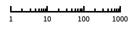
自動目盛ラベル付きの対数スケール "Log10" 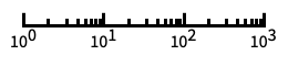
10のベキ乗に目盛が付いた,10を底とする対数スケール "SignedLog" 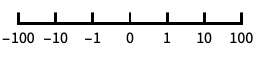
0と負の数を含む対数に似たスケール "Reverse" 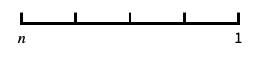
座標の向きを逆にする "Infinite" 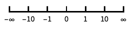
無限スケール
全オプションのリスト
例題
すべて開く すべて閉じる例 (1)
data = ExampleData[{"Geometry3D", "StanfordBunny"}, "VertexData"];ListSurfacePlot3D[data, MaxPlotPoints -> 50]ListSurfacePlot3D[data, MaxPlotPoints -> 50, Mesh -> 30, Axes -> None, MeshFunctions -> (#1 - #2 + #3&), MeshShading -> {None, Automatic}]スコープ (13)
データ (4)
data = Table[{Sin[u], Cos[u], Sqrt[Cos[u]]}, {u, 0, 2Pi, 0.1}];ListPointPlot3D[data, BoxRatios -> 1]ListSurfacePlot3D[data, BoxRatios -> 1]MaxPlotPointsを使って使用する点の数を制限する:
data = Table[Block[{x = RandomReal[{-1, 1}], y = RandomReal[{-1, 1}]}, {x, y, RandomChoice[{-1, 1}]Sqrt[1 - x ^ 2 - y ^ 2]}RandomReal[{0.95, 1.05}]], {2000}];Table[ListSurfacePlot3D[data, MaxPlotPoints -> mp, Mesh -> All], {mp, {50, 25, 10, Infinity}}]PlotRangeを使って興味のある部分に焦点を当てる:
data = ExampleData[{"Geometry3D", "StanfordBunny"}, "VertexData"];{ListSurfacePlot3D[data, Mesh -> None, MaxPlotPoints -> 35], ListSurfacePlot3D[data, Mesh -> None, MaxPlotPoints -> 35, PlotRange -> {{-0.1, -0.02}, All, {0.1, 0.2}}]}RegionFunctionを使って曲面を不等式によって与えられる範囲に制限する:
data = ExampleData[{"Geometry3D", "StanfordBunny"}, "VertexData"];ListSurfacePlot3D[data, Mesh -> None, MaxPlotPoints -> 35, PlotStyle -> FaceForm[Yellow, Cyan], RegionFunction -> Function[{x, y, z}, Norm[{x - 0, z - 0.1}] ≥ 0.035]]表形式データ (1)
プレゼンテーション (8)
明示的なPlotStyleを曲面に与える:
data = ExampleData[{"Geometry3D", "StanfordBunny"}, "VertexData"];ListSurfacePlot3D[data, Mesh -> None, MaxPlotPoints -> 35, PlotStyle -> Directive[Purple, Specularity[White, 10]]]data = ExampleData[{"Geometry3D", "Torus"}, "VertexData"];ListSurfacePlot3D[data, MaxPlotPoints -> 35, Mesh -> None, PlotLabel -> "torus", AxesLabel -> {x, y, z}, Ticks -> None]data = ExampleData[{"Geometry3D", "StanfordBunny"}, "VertexData"];ListSurfacePlot3D[data, Mesh -> None, MaxPlotPoints -> 35, ColorFunction -> Function[{x, y, z}, ColorData["GreenBrownTerrain"][z]]]data = ExampleData[{"Geometry3D", "Torus"}, "VertexData"];ListSurfacePlot3D[data, MaxPlotPoints -> 35, Axes -> False, Mesh -> 35, MeshStyle -> Thick, MeshFunctions -> {Function[{x, y, z}, ArcTan[x, y]]}, PlotStyle -> Pink]data = ExampleData[{"Geometry3D", "StanfordBunny"}, "VertexData"];ListSurfacePlot3D[data, Mesh -> 12, MaxPlotPoints -> 35, ColorFunction -> (Hue[Sin[10#1]Sin[10#2]]&), MeshShading -> {{{StandardGray, Automatic}, {Automatic, StandardGray}}, {{Automatic, StandardGray}, {StandardGray, Automatic}}}]data = ExampleData[{"Geometry3D", "StanfordBunny"}, "VertexData"];ListSurfacePlot3D[data, MaxPlotPoints -> 35, PlotTheme -> "Marketing"]data = ExampleData[{"Geometry3D", "StanfordBunny"}, "VertexData"];ListSurfacePlot3D[data, MaxPlotPoints -> 35, PlotTheme -> "Minimal"]ScalingFunctionsを使って x 軸を反転させる:
ListSurfacePlot3D[ExampleData[{"Geometry3D", "StanfordBunny"}, "VertexData"], MaxPlotPoints -> 50, ScalingFunctions -> {"Reverse", None, None}]オプション (70)
Axes (3)
デフォルトで,Axesが描かれる:
ListSurfacePlot3D[IconizedObject[«data»]]ListSurfacePlot3D[IconizedObject[«data»], Axes -> False]{ListSurfacePlot3D[IconizedObject[«data»], Axes -> {True, False, False}], ListSurfacePlot3D[IconizedObject[«data»], Axes -> {False, True, False}], ListSurfacePlot3D[IconizedObject[«data»], Axes -> {False, False, True}]}AxesLabel (4)
ListSurfacePlot3D[IconizedObject[«data»]]
ListSurfacePlot3D[IconizedObject[«data»], AxesLabel -> z]ListSurfacePlot3D[IconizedObject[«data»], AxesLabel -> {x, y, z}]ListSurfacePlot3D[QuantityArray[IconizedObject[«data»], "Meters"], AxesLabel -> Automatic]AxesOrigin (2)
AxesStyle (4)
ListSurfacePlot3D[IconizedObject[«data»], AxesStyle -> Red]ListSurfacePlot3D[IconizedObject[«data»], AxesStyle -> {{Thick, Brown}, {Thick, Blue}, {Thick, Green}}]ListSurfacePlot3D[IconizedObject[«data»], AxesStyle -> Green, TicksStyle -> StandardBlue]ListSurfacePlot3D[IconizedObject[«data»], AxesStyle -> Green, LabelStyle -> StandardBlue]BoundaryStyle (4)
data = Flatten[Table[{Cos[ϕ] θ, Sin[ϕ] θ, 2 - θ}, {ϕ, 0., 2Pi, 0.2}, {θ, 0.5, 1.5, 0.1}], 1];ListSurfacePlot3D[data, Mesh -> None]data = Flatten[Table[{Cos[ϕ] θ, Sin[ϕ] θ, 2 - θ}, {ϕ, 0., 2Pi, 0.2}, {θ, 0.5, 1.5, 0.1}], 1];ListSurfacePlot3D[data, Mesh -> None, BoundaryStyle -> Thick]data = Flatten[Table[{Cos[ϕ] θ, Sin[ϕ] θ, 2 - θ}, {ϕ, 0., 2Pi, 0.2}, {θ, 0.5, 1.5, 0.1}], 1];ListSurfacePlot3D[data, Mesh -> None, BoundaryStyle -> Directive[Red, Thick]]BoundaryStyleはRegionFunctionによって切り取られた穴に適用される:
data = Flatten[Table[{Cos[ϕ] θ, Sin[ϕ] θ, 2 - θ}, {ϕ, 0., 2Pi, 0.2}, {θ, 0.5, 1.5, 0.1}], 1];ListSurfacePlot3D[data, Mesh -> None, BoundaryStyle -> Thick, RegionFunction -> Function[{x, y, z}, z > 1.25 || z < 0.75], PlotRange -> All]ColorFunction (4)


data = ExampleData[{"Geometry3D", "StanfordBunny"}, "VertexData"];Table[ListSurfacePlot3D[data, Mesh -> None, MaxPlotPoints -> 35, ColorFunction -> Function[{x, y, z}, Evaluate[f]], PlotLabel -> f, Axes -> False], {f, {Hue[x], Hue[y], Hue[z]}}]
data = ExampleData[{"Geometry3D", "StanfordBunny"}, "VertexData"];ListSurfacePlot3D[data, Mesh -> None, MaxPlotPoints -> 35, ColorFunction -> "Rainbow"]ColorFunctionはPlotStyleよりも優先順位が高い:
data = ExampleData[{"Geometry3D", "StanfordBunny"}, "VertexData"];ListSurfacePlot3D[data, Mesh -> None, MaxPlotPoints -> 35, ColorFunction -> "Rainbow", PlotStyle -> Directive[Opacity[0.5], Red]]ColorFunctionはMeshShadingよりも優先順位が低い:
data = ExampleData[{"Geometry3D", "StanfordBunny"}, "VertexData"];ListSurfacePlot3D[data, MaxPlotPoints -> 35, ColorFunction -> (Hue[#3]&), Mesh -> 8, MeshShading -> {{{None, Automatic}, {Automatic, None}}, {{Automatic, None}, {None, Automatic}}}]ColorFunctionScaling (1)
data = ExampleData[{"Geometry3D", "StanfordBunny"}, "VertexData"];ListSurfacePlot3D[data, Mesh -> None, MaxPlotPoints -> 50, ColorFunction -> Function[{x, y, z}, ColorData["DarkBands"][Rescale[Sin[50x]Sin[50y]Sin[50z], {-1, 1}]]], ColorFunctionScaling -> False]ImageSize (7)
Tiny,Small,Medium,Largeのような名前付きのサイズを使う:
{ListSurfacePlot3D[IconizedObject[«data»], ImageSize -> Tiny], ListSurfacePlot3D[IconizedObject[«data»], ImageSize -> Small]}{ListSurfacePlot3D[IconizedObject[«data»], ImageSize -> 150], ListSurfacePlot3D[IconizedObject[«data»], AspectRatio -> 1.5, ImageSize -> 150]}{ListSurfacePlot3D[IconizedObject[«data»], ImageSize -> {Automatic, 150}], ListSurfacePlot3D[IconizedObject[«data»], AspectRatio -> 2, ImageSize -> {Automatic, 150}]}{ListSurfacePlot3D[IconizedObject[«data»], ImageSize -> UpTo[200]], ListSurfacePlot3D[IconizedObject[«data»], AspectRatio -> 2, ImageSize -> UpTo[200]]}グラフィックスの幅と高さを指定して,必要な場合はスペースで充填する:
ListSurfacePlot3D[IconizedObject[«data»], ImageSize -> {200, 300}, Background -> StandardGray]AspectRatioFullと設定すると,使用可能なスペースが塗り潰される:
ListSurfacePlot3D[IconizedObject[«data»], AspectRatio -> Full, ImageSize -> {200, 300}, Background -> StandardGray]{ListSurfacePlot3D[IconizedObject[«data»], ImageSize -> {UpTo[150], UpTo[100]}], ListSurfacePlot3D[IconizedObject[«data»], AspectRatio -> 2, ImageSize -> {UpTo[150], UpTo[100]}]}ImageSizeFullを使ってオブジェクト内の使用可能なスペースを塗り潰す:
Framed[Pane[ListSurfacePlot3D[IconizedObject[«data»], ImageSize -> Full, Background -> StandardGray], {200, 100}]]Framed[Pane[ListSurfacePlot3D[IconizedObject[«data»], AspectRatio -> Full, ImageSize -> {Scaled[0.5], Scaled[0.5]}, Background -> StandardGray], {200, 200}]]Mesh (5)
data = ExampleData[{"Geometry3D", "Torus"}, "VertexData"];ListSurfacePlot3D[data, MaxPlotPoints -> 35, Mesh -> None]data = ExampleData[{"Geometry3D", "Torus"}, "VertexData"];ListSurfacePlot3D[data, MaxPlotPoints -> 35, Mesh -> All]data = ExampleData[{"Geometry3D", "Torus"}, "VertexData"];ListSurfacePlot3D[data, MaxPlotPoints -> 35, Mesh -> 5]3本のメッシュラインを  方向に,6本のメッシュラインを
 方向に使う:
data = ExampleData[{"Geometry3D", "Torus"}, "VertexData"];ListSurfacePlot3D[data, MaxPlotPoints -> 35, Mesh -> {3, 6}, MeshFunctions -> {#1&, #2&}]data = ExampleData[{"Geometry3D", "Torus"}, "VertexData"];ListSurfacePlot3D[data, Mesh -> {{1, 2}, {Pi / 2}, {0}}]MeshFunctions (2)


data = ExampleData[{"Geometry3D", "Torus"}, "VertexData"];Table[ListSurfacePlot3D[data, MaxPlotPoints -> 35, Axes -> False, Mesh -> 15, MeshFunctions -> {Function[{x, y, z}, Evaluate[f]]}, PlotLabel -> f], {f, {x, y, z}}]data = ExampleData[{"Geometry3D", "Torus"}, "VertexData"];ListSurfacePlot3D[data, MaxPlotPoints -> 35, Axes -> False, Mesh -> 15, MeshFunctions -> {Function[{x, y, z}, ArcTan[x, y]]}]MeshShading (4)
Noneを使って領域を取り除く:
data = ExampleData[{"Geometry3D", "StanfordBunny"}, "VertexData"];ListSurfacePlot3D[data, Mesh -> 15, MaxPlotPoints -> 35, MeshFunctions -> {#3&}, MeshShading -> {FaceForm[Red, Yellow], None}]data = ExampleData[{"Geometry3D", "StanfordBunny"}, "VertexData"];ListSurfacePlot3D[data, Mesh -> 10, MaxPlotPoints -> 35, MeshFunctions -> {#1&, #2&}, MeshShading -> {{Yellow, Green}, {Green, Yellow}}]MeshShadingはPlotStyleよりも優先順位が高い:
data = ExampleData[{"Geometry3D", "StanfordBunny"}, "VertexData"];ListSurfacePlot3D[data, Mesh -> 10, MaxPlotPoints -> 35, MeshFunctions -> {#1&, #2&}, PlotStyle -> Red, MeshShading -> {{Green, Automatic}, {Automatic, Green}}]MeshShadingはColorFunctionよりも優先順位が高い:
data = ExampleData[{"Geometry3D", "StanfordBunny"}, "VertexData"];ListSurfacePlot3D[data, Mesh -> 10, MaxPlotPoints -> 35, MeshFunctions -> {#1&, #2&}, MeshShading -> {{StandardGray, Automatic}, {Automatic, StandardGray}}, ColorFunction -> "DarkRainbow"]MeshStyle (2)
data = ExampleData[{"Geometry3D", "Torus"}, "VertexData"];ListSurfacePlot3D[data, MaxPlotPoints -> 35, Mesh -> 5, MeshStyle -> Red] 方向に赤いメッシュラインを,
 方向に青いメッシュラインを,
 方向に太いメッシュラインを使う:
data = ExampleData[{"Geometry3D", "Torus"}, "VertexData"];ListSurfacePlot3D[data, MaxPlotPoints -> 35, Mesh -> 5, MeshStyle -> {Red, Blue, Thick}]PlotStyle (6)
data = ExampleData[{"Geometry3D", "StanfordBunny"}, "VertexData"];ListSurfacePlot3D[data, Mesh -> None, MaxPlotPoints -> 35, PlotStyle -> Cyan]Specularityでハイライト効果を得る:
data = ExampleData[{"Geometry3D", "StanfordBunny"}, "VertexData"];ListSurfacePlot3D[data, Mesh -> None, MaxPlotPoints -> 35, PlotStyle -> Directive[Cyan, Specularity[White, 10]]]Opacityを使って透過性のある表面にする:
data = ExampleData[{"Geometry3D", "StanfordBunny"}, "VertexData"];ListSurfacePlot3D[data, Mesh -> None, MaxPlotPoints -> 35, PlotStyle -> Directive[Cyan, Opacity[0.5]]]data = ExampleData[{"Geometry3D", "StanfordBunny"}, "VertexData"];ListSurfacePlot3D[data, MaxPlotPoints -> 35, PlotStyle -> None]ColorFunctionはPlotStyleよりも優先順位が高い:
data = ExampleData[{"Geometry3D", "StanfordBunny"}, "VertexData"];ListSurfacePlot3D[data, Mesh -> None, MaxPlotPoints -> 35, ColorFunction -> "Rainbow", PlotStyle -> Directive[Opacity[0.5], Cyan]]MeshShadingはPlotStyleよりも優先順位が高い:
data = ExampleData[{"Geometry3D", "StanfordBunny"}, "VertexData"];ListSurfacePlot3D[data, Mesh -> 10, MaxPlotPoints -> 35, MeshFunctions -> {#1&, #2&}, PlotStyle -> Cyan, MeshShading -> {{StandardGray, Automatic}, {Automatic, StandardGray}}]PlotTheme (1)
RegionFunction (3)


data = Table[Block[{x = RandomReal[{-1, 1}], y = RandomReal[{-1, 1}]}, {x, y, RandomChoice[{-1, 1}]Sqrt[1 - x ^ 2 - y ^ 2]}], {2000}];Table[ListSurfacePlot3D[data, Mesh -> None, RegionFunction -> Function[{x, y, z}, Evaluate[f]], PlotLabel -> f, AxesEdge -> {{-1, 0}, {1, 0}, {-1, 0}}], {f, {Abs[x] > 0.25, Abs[y] > 0.25, Abs[z] > 0.25}}]
data = ExampleData[{"Geometry3D", "StanfordBunny"}, "VertexData"];ListSurfacePlot3D[data, Mesh -> None, MaxPlotPoints -> 35, RegionFunction -> Function[{x, y, z}, x < y]]ScalingFunctions (4)
ListSurfacePlot3D[Flatten[Table[{Cos[ϕ] θ, Sin[ϕ] θ, 3θ}, {ϕ, 0., 2Pi, 0.1}, {θ, 0.5, Pi, 0.1}], 1], BoxRatios -> {1, 1, 1}]対数スケールのプロットはLogが定義された領域しかプロットしない:
ListSurfacePlot3D[Flatten[Table[{Cos[ϕ] θ, Sin[ϕ] θ, 3θ}, {ϕ, 0., 2Pi, 0.1}, {θ, 0.5, Pi, 0.1}], 1], ScalingFunctions -> {None, None, "Log"}, BoxRatios -> {1, 1, 1}]シフトされた対数スケールを使って負の値がある関数を表示する:
ListSurfacePlot3D[Flatten[Table[{Cos[ϕ] θ, Sin[ϕ] θ, 3θ}, {ϕ, 0., 2Pi, 0.1}, {θ, 0.5, Pi, 0.1}], 1], ScalingFunctions -> {None, None, "SignedLog"}, BoxRatios -> {1, 1, 1}]ScalingFunctionsを使って  方向の座標方向を逆にする:
ListSurfacePlot3D[Flatten[Table[{Cos[ϕ] θ, Sin[ϕ] θ, 3θ - 3}, {ϕ, 0., 2Pi, 0.1}, {θ, 0.5, Pi, 0.1}], 1], ScalingFunctions -> {None, None, "Reverse"}, BoxRatios -> {1, 1, 1}]TextureCoordinateFunction (4)


data = ExampleData[{"Geometry3D", "StanfordBunny"}, "VertexData"];ListSurfacePlot3D[data, Mesh -> None, MaxPlotPoints -> 35, PlotStyle -> Texture[ExampleData[{"ColorTexture", "CheetahFur"}]]]

data = ExampleData[{"Geometry3D", "StanfordBunny"}, "VertexData"];ListSurfacePlot3D[data, Mesh -> None, MaxPlotPoints -> 35, TextureCoordinateFunction -> ({#1, #3}&), PlotStyle -> Texture[ExampleData[{"ColorTexture", "CheetahFur"}]]]data = ExampleData[{"Geometry3D", "StanfordBunny"}, "VertexData"];ListSurfacePlot3D[data, MaxPlotPoints -> 35, Mesh -> None, TextureCoordinateScaling -> False, PlotStyle -> Texture[ExampleData[{"ColorTexture", "CheetahFur"}]]]テクスチャを使ってパラメータがどのように曲面にマップされるかをハイライトする:
texture = ArrayPlot[{{1, 1, 1, 2, 1, 1}, {2, 0, 0, 2, 0, 0}, {2, 0, 0, 2, 0, 0}, {2, 1, 1, 1, 1, 1}, {2, 0, 0, 2, 0, 0}, {2, 0, 0, 2, 0, 0}}, ColorRules -> {1 -> Red, 2 -> Blue, 0 -> White}, Frame -> False, PlotRangePadding -> None, ImagePadding -> None, ImageSize -> 100]data = ExampleData[{"Geometry3D", "StanfordBunny"}, "VertexData"];ListSurfacePlot3D[data, Mesh -> None, MaxPlotPoints -> 35, PlotStyle -> Texture[texture]]TextureCoordinateScaling (1)
テクスチャにスケールされたあるいはスケールされていない座標を使う:
texture = ArrayPlot[{{1, 1, 1, 2, 1, 1}, {2, 0, 0, 2, 0, 0}, {2, 0, 0, 2, 0, 0}, {2, 1, 1, 1, 1, 1}, {2, 0, 0, 2, 0, 0}, {2, 0, 0, 2, 0, 0}}, ColorRules -> {1 -> Red, 2 -> Blue, 0 -> White}, Frame -> False, PlotRangePadding -> None, ImagePadding -> None, ImageSize -> 100]data = ExampleData[{"Geometry3D", "StanfordBunny"}, "VertexData"];Table[ListSurfacePlot3D[data, Mesh -> None, MaxPlotPoints -> 35, TextureCoordinateScaling -> s, PlotStyle -> Texture[texture], PlotLabel -> s], {s, {True, False}}]Ticks (6)
ListSurfacePlot3D[ExampleData[{"Geometry3D", "StanfordBunny"}, "VertexData"], MaxPlotPoints -> 35]ListSurfacePlot3D[ExampleData[{"Geometry3D", "StanfordBunny"}, "VertexData"], MaxPlotPoints -> 35, Ticks -> None]ListSurfacePlot3D[ExampleData[{"Geometry3D", "StanfordBunny"}, "VertexData"], MaxPlotPoints -> 35, Ticks -> {{-.07, 0, .05}, {-.05, 0, .05}, {.04, .09, .15}}]ListSurfacePlot3D[ExampleData[{"Geometry3D", "StanfordBunny"}, "VertexData"], MaxPlotPoints -> 35, Ticks -> {{{-.05, -a}, {0, 0}, {.05, a}}, {{-.05, -a}, {0, 0}, {.05, a}}, {{.04, b}, {.09, c}, {.15, d}}}]ListSurfacePlot3D[ExampleData[{"Geometry3D", "StanfordBunny"}, "VertexData"], MaxPlotPoints -> 35, Ticks -> {{{-.05, -a, .05}, {0, 0, .05}, {.05, a, .05}}, {{-.05, -a, .1}, {0, 0, .1}, {.05, a, .1}}, {{.04, b, .22}, {.09, c, .2}, {.15, d, .07}}}]ListSurfacePlot3D[ExampleData[{"Geometry3D", "StanfordBunny"}, "VertexData"], MaxPlotPoints -> 35, Ticks -> {{{-.05, -a, .05, Directive[Red]}, {0, 0, .05, Directive[Red, Thick]}, {.05, a, .05, Directive[Red, Thick]}}, {{-.05, -a, .1, Directive[Blue]}, {0, 0, .1, Directive[Blue]}, {.05, a, .1, Directive[Blue, Thick]}}, {{.04, b, .22, Directive[Brown, Thick]}, {.09, c, .2, Directive[Brown, Dashed, Thick]}, {.15, d, .07, Directive[Orange, Thick]}}}]TicksStyle (3)
デフォルトで,目盛と目盛ラベルには軸と同じスタイルが使われる:
ListSurfacePlot3D[ExampleData[{"Geometry3D", "StanfordBunny"}, "VertexData"], MaxPlotPoints -> 35, AxesStyle -> Directive[Blue, Thick]]ListSurfacePlot3D[ExampleData[{"Geometry3D", "StanfordBunny"}, "VertexData"], MaxPlotPoints -> 35, TicksStyle -> Directive[Blue, Thick]]ListSurfacePlot3D[ExampleData[{"Geometry3D", "StanfordBunny"}, "VertexData"], MaxPlotPoints -> 35, TicksStyle -> {Directive[Blue, Thick], Directive[Darker@Green, Thick], Directive[Red, Thick]}]アプリケーション (1)
ListSurfacePlot3D[Flatten[Table[{Cos[ϕ] Sin[θ], Sin[θ] Sin[ϕ], Cos[θ]}, {ϕ, -π, π, .2}, {θ, 0, π, .2}], 1]]ListSurfacePlot3D[Flatten[Table[{Cos[ϕ] Sin[θ], Sin[θ] Sin[ϕ], Cos[θ]} + RandomReal[.1, 3], {ϕ, -π, π, .2}, {θ, 0, π, .2}], 1]]特性と関係 (13)
ListPlot3Dは常に1枚のシートで関数の曲面を推測する:
data = Flatten[Table[{v Sin[u], v Cos[u], u}, {u, 0, 2Pi, 0.1}, {v, 0, 1, .2}], 1];ListPlot3D[data, BoxRatios -> 1]ListSurfacePlot3Dは何枚のシートでも埋めることができる:
ListSurfacePlot3D[data, BoxRatios -> 1]ListSurfacePlot3Dは近似した一般的な曲面を作成する:
data1 = Flatten[Table[{Cos[ϕ] Sin[θ], Sin[ϕ] Sin[θ], -Cos[θ]}, {ϕ, 0., 2Pi, 0.4}, {θ, 0., Pi, 0.4}], 1];ListSurfacePlot3D[data1, Mesh -> All]ListPlot3Dは  方向に急速に振動する関数曲面を作成する:
ListPlot3D[data1, BoxRatios -> Automatic, Mesh -> None]各  ,
 値に対して複数の
 値を使うと,ListPlot3Dによって重複が無視される:
data2 = Flatten[Table[{Cos[ϕ] Sin[θ], Sin[ϕ] Sin[θ], Cos[θ]}, {ϕ, 0., 2Pi, (2Pi) / 25}, {θ, 0., Pi, Pi / 25}], 1];ListPlot3D[data2, BoxRatios -> Automatic, Mesh -> None]ListSurfacePlot3Dはそれでも一般的な曲面を再構築する:
ListSurfacePlot3D[data2]ListPointPlot3Dを使って三次元の点を示す:
ListPointPlot3D[Table[Sin[j ^ 2 + i], {i, 0, Pi, 0.1}, {j, 0, Pi, 0.1}]]ListContourPlot3Dを使って  ,
 ,
 データに関連した値を通る等高線を求める:
data = Table[Append[pt, Norm[pt]], {pt, RandomReal[1, {5000, 3}]}];ListContourPlot3D[data]ListContourPlotを使って連続データから等高線を作成する:
ListContourPlot[Table[Sin[j ^ 2 + i], {i, 0, Pi, 0.1}, {j, 0, Pi, 0.1}]]ListDensityPlotを使って連続データから密度を作成する:
ListDensityPlot[Table[Sin[j ^ 2 + i], {i, 0, Pi, 0.1}, {j, 0, Pi, 0.1}]]離散データの配列にArrayPlotを使う:
ArrayPlot[CellularAutomaton[30, {{1}, 0}, 50]]行列の構造化プロットにMatrixPlotを使う:
MatrixPlot[Import[ "ExampleData/bcsstk08.mtx.gz"]]ReliefPlotを医学および地理学の値に対応する行列に使う:
ReliefPlot[Import["http://exampledata.wolfram.com/hailey.dem.gz", "Data"], ColorFunction -> "GreenBrownTerrain", MaxPlotPoints -> 200]ListLogPlot,ListLogLogPlot,ListLogLinearPlotを対数プロットに使う:
ListLogPlot[Table[Fibonacci[k], {k, 0, 15}], Joined -> True]ListPolarPlotを極プロットに使う:
ListPolarPlot[Table[{x, Sqrt[x]}, {x, 0, 2Pi, 0.1}]]DateListPlotを使って時間に沿ったデータを示す:
DateListPlot[{5, 11, 13, 24, 28, 31, 34, 39, 42, 47, 51, 66}, {2006, 1}, PlotStyle -> PointSize[Medium]]ParametricPlot3Dを三次元パラメトリック曲線と曲面に使う:
{ParametricPlot3D[{Cos[θ], Sin[θ], Sqrt[θ]}, {θ, 0, 6Pi}], ParametricPlot3D[{r ^ 2 Cos[θ], r ^ 2 Sin[θ], r Sqrt[θ]}, {r, 0, 1}, {θ, 0, 6Pi}]}テキスト
Wolfram Research (2007), ListSurfacePlot3D, Wolfram言語関数, https://reference.wolfram.com/language/ref/ListSurfacePlot3D.html (2025年に更新).
CMS
Wolfram Language. 2007. "ListSurfacePlot3D." Wolfram Language & System Documentation Center. Wolfram Research. Last Modified 2025. https://reference.wolfram.com/language/ref/ListSurfacePlot3D.html.
APA
Wolfram Language. (2007). ListSurfacePlot3D. Wolfram Language & System Documentation Center. Retrieved from https://reference.wolfram.com/language/ref/ListSurfacePlot3D.html