



Histogram
詳細とオプション
- Histogram[data]は,デフォルトで,仮定される値 xiのもとになっている滑らかな分布を近似するために選ばれた等しいビン幅でヒストグラムをプロットする.
- データ値 xiは次の形式で与えることができる.
-
xi 数 Quantity[xi,unit] 単位の付いた数 - データ集合 dataiには,次の形式と解釈がある.
-
{x1,x2,…} 値 xiのリスト <k1x1,k2x2,…> 連想からの値 xi QuantityArray 大きさ TimeSeries,EventSeries,… 時系列データからの値 WeightedData 各値の数はその重みである w[datai] データ集合 dataiにラッパー w - Histogram[objcspec]は,列指定 cspec を用いて,Tabular,TimeSeriesまたはEventSeriesの各オブジェクト obj から値を抽出してプロットする.
- 表形式データをプロットには,以下の指定 cspec が使用できる.
-
col キー col からのヒストグラム値 {col1,col2,…} キー col1,col2,…からのヒストグラム値 - 使用可能なビン幅指定 bspec
-
n n 個のビンを使う {dx} 幅が dx のビンを使う {xmin,xmax,dx} xminから xmaxまでの幅 dx のビンを使う {{b1,b2,…}} ビン[b1,b2),[b2,b3),…を使う Automatic ビン幅を自動的に決定する "name" 名前付きのビンメソッドを使う {"Log",bspec} ビン bspec を対数変換されたデータに適用する fb 明示的なビン指定{b1,b2,…}を得るために fb を適用する - ビン指定"Log"はもとのビンメソッドAutomaticを使うものと解釈される.
- 使用可能な名前付きビンメソッド
-
"Sturges" データの長さに基づいたビンの数を計算する "Scott" 平均二乗誤差を漸近的に最小化する "FreedmanDiaconis" 四分位範囲をサンプルサイズの立方根で割ったものの2倍 "Knuth" 区分一様モデルの平衡尤度と事前確率 "Wand" 1レベル再帰的に近似したWandのビンメソッド - Histogram[data,fb]の関数 fb はすべての xiのリストに適用され,明示的なビンリスト{b1,b2,…}を返す.
- Histogram[data,bspec,hspec]でのビンの高さ指定 hspec を変えることで,異なる形式のヒストグラムを得ることができる.次は使用可能な形式である.
-
"Count" 各ビンに入る値の数 "CumulativeCount" 累積数 "SurvivalCount" 残存数 "Probability" 各ビンに入る値の割合 "Intensity" ビン幅で区切られた数 "PDF" 確率密度関数 "CDF" 累積分布関数 "SF" 生存関数 "HF" ハザード関数 "CHF" 累積ハザード関数 {"Log",hspec} 対数変換された高さの指定 fh fh をビンと数に適用して得られた高さ - Histogram[data,bspec,fh]の関数 fh はビンのリスト{{b1,b2},{b2,b3},…}と対応する数のリスト{c1,c2,…}の2つの引数に適用される.この関数は各 ciに使用される高さのリストを返す.
- ビンには実数値 xiのみを割り当てることができる.その他の値の場合は欠測値とみなされる.
- Histogram[{data1,data2,…},…]では,すべてのデータ集合 dataiを組み合せることで自動的にビン位置が決定される.
- Histogram[{…,wi[datai,…],…},…]は,記号的ラッパー wiによって定義された指定に従ってデータ集合 dataiに関連したヒストグラム要素を描画する.
- 次は,グラフ要素に使えるラッパーである.
-
Annotation[e,label] 注釈を与える Button[e,action] 要素がクリックされたときに実行するアクションを定義する Callout[e,label] 要素にコールアウトを付けて表示する EventHandler[e,…] 要素の一般的なイベントハンドラを定義する Hyperlink[e,uri] 要素をハイパーリンクにする Labeled[e,…] 要素にラベルを付けて表示する Legended[e,…] グラフの凡例に要素の特徴を含める Mouseover[e,over] 要素がマウスオーバー形式を表示するようにする PopupWindow[e,cont] 要素にポップアップウィンドウを付ける StatusArea[e,label] 要素のマウスオーバー時にステータスエリアに表示する Style[e,opts] 要素を指定のスタイルで表示する Tooltip[e,label] 要素に任意のツールチップを付ける - HistogramにはGraphicsと同じオプションに以下の追加・変更を加えたものが使える. [全オプションのリスト]
-
AspectRatio 1/GoldenRatio 縦横比 Axes True 軸を描くかどうか BarOrigin Bottom ヒストグラムの棒の始点 ChartBaseStyle Automatic 棒の全体的なスタイル ChartElementFunction Automatic 棒の生のグラフィックスをどのように生成するか ChartElements Automatic 各棒に使うグラフィックス ColorFunction Automatic 棒の彩色方法 ColorFunctionScaling True ColorFunctionの引数を正規化するかどうか LabelingFunction Automatic 要素にどのようにラベルを付けるか LegendAppearance Automatic 凡例の全体的な外観 PerformanceGoal $PerformanceGoal パフォーマンスのどの面について最適化するか PlotFit None 曲線をヒストグラムにどのようにフィットするか PlotFitElements Automatic ヒストグラム内に表示するフィットされた要素 PlotInteractivity $PlotInteractivity インタラクティブ要素を許可するかどうか PlotLabels None データ集合のカテゴリラベル PlotLayout Automatic 使用する全体的なレイアウト PlotLegends None データ要素とデータ集合の凡例 PlotStyle Automatic 棒のスタイル PlotTheme $PlotTheme ヒストグラムの全体的なテーマ ScalingFunctions None 個々の座標をどのようにスケールするか TargetUnits Automatic グラフ内に表示する単位 - 複数のデータ集合は,PlotLayoutの次の設定を使って表示できる.
-
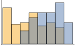
"Overlapped" 全データを重ね合せて表示する 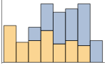
"Stacked" ビンごとにデータを積み重ねる - 次は,複数のパネルのそれぞれに単一の棒のグループを表示するPlotLayoutの可能な設定である.
-
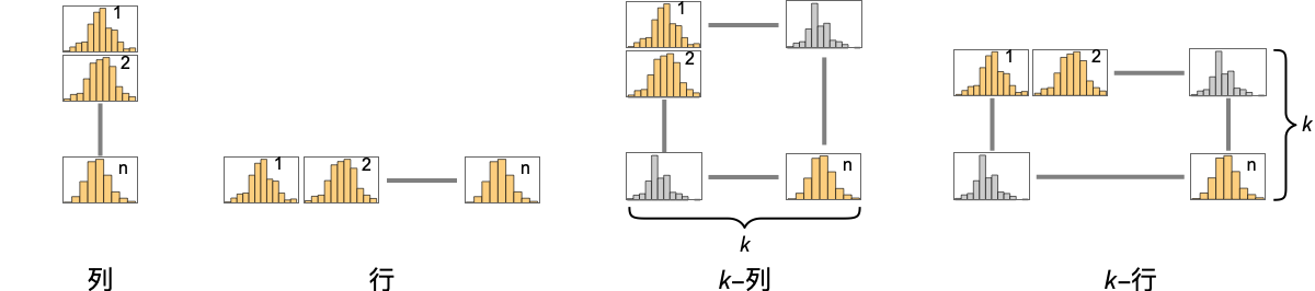
"Column" パネルの列に別々の棒のグループを使う "Row" パネルの行に別々の棒のグループを使う {"Column",k},{"Row",k} k 列(または行)を使う {"Column",UpTo[k]},{"Row",UpTo[k]} 最大で k 列(または行)を使う - PlotLegendsの典型的な設定には以下がある.
-
None 凡例なし Automatic 凡例を自動的に決定する {lbl1,lbl2,…} lbl1,lbl2,…を凡例ラベルとして用いる Placed[lspec,…] 凡例の配置を指定する - PlotStylesty は各曲線に使用するスタイルを指定する.可能な設定には以下が含まれる.
-
{sty1,sty2,…} データ集合に対するスタイルの並び <"key"val,…> データの異なるレベルに対するスタイル要素 - 使用可能なキーは次の通りである.
-
"Base" すべての dataiに対する全体的なスタイル "Lists" dataiごとのスタイル styiのリスト - ColorData["DefaultChartColors"]は,PlotStyleで用いられるデフォルトの色の並びを与える.
- ChartElementFunctionに渡される引数は,データ集合のネストしたリストの各レベルからのビンの範囲{{xmin,xmax},{ymin,ymax}},ビンの値 lists,メタデータ{m1,m2,…}である.
- ChartElementFunctionの組込み設定のリストはChartElementData["Histogram"]で得ることができる.
- ColorFunctionに渡される引数は各ビンの高さである.
- ScalingFunctions->{sx,sy}では,
 座標は sx等を使ってスケールされる.
- BarChart内のオプションその他の構造からのスタイルその他の指定は,事実上PlotStyle,ColorFunction,Styleその他のラッパー,ChartElementsおよびChartElementFunctionの順に適用される.後ろの指定が前方の指定を無効にする.
全オプションのリスト
例題
すべて開く すべて閉じる例 (4)
Histogram[RandomVariate[NormalDistribution[0, 1], 200]]data1 = RandomVariate[NormalDistribution[0, 1], 500];
data2 = RandomVariate[NormalDistribution[3, 1 / 2], 500];Histogram[{data1, data2}]Histogram[RandomVariate[WeibullDistribution[2, 1], 1000], Automatic, "Probability"]Histogram[{IconizedObject[«data1»], IconizedObject[«data2»]}, PlotLayout -> "Row"]スコープ (35)
データとレイアウト (19)
data = RandomVariate[NormalDistribution[0, 1], 200];Histogram[data, 5]Histogram[data, {.5}]Histogram[data, {-2, 2, 1}]Histogram[data, {{-3, -1, 0, 1, 3}}]Histogram[RandomInteger[10, 250]]data = RandomVariate[NormalDistribution[0, 1], 1000];Table[Histogram[data, b, PlotLabel -> b], {b, {"Sturges", "Scott", "FreedmanDiaconis", "Wand"}}]Histogram[data, "Log"]integerBins[list_] := Union[IntegerPart[list]]integerBins[{1.2, 1.8, 2.3, 2.5}]Histogram[RandomReal[20, 100], integerBins]data = RandomVariate[NormalDistribution[0, 1], 200];Table[Histogram[data, Automatic, h, PlotLabel -> h], {h, {"Count", "Probability", "PDF", "CumulativeCount", "CDF", "SF"}}]accumulatedCount[bins_, counts_] := Accumulate[counts]Histogram[RandomVariate[NormalDistribution[0, 1], 200], Automatic, accumulatedCount]data1 = RandomVariate[NormalDistribution[0, 1], 500];
data2 = RandomVariate[NormalDistribution[3, 1 / 2], 500];
data3 = RandomVariate[NormalDistribution[5, 1 / 3], 500];Histogram[{data1, data2, data3}]Histogram[{1, 2, 3, None, 3, 5, Missing[], 2, 1, foo, 2, 3}]data1 = RandomVariate[NormalDistribution[0, 1], 500];
data2 = RandomVariate[NormalDistribution[3, 1 / 2], 500];Histogram[{data1, None, data2}]Histogram[{Quantity[1, "Meters"], Quantity[3, "Meters"], Quantity[2, "Meters"], Quantity[2, "Meters"], Quantity[3, "Meters"], Quantity[2, "Meters"], Quantity[5, "Meters"], Quantity[3, "Meters"], Quantity[2, "Meters"], Quantity[4, "Meters"]}, AxesLabel -> Automatic]Histogram[{Quantity[1, "Meters"], Quantity[3, "Meters"], Quantity[2, "Meters"], Quantity[2, "Meters"], Quantity[3, "Meters"], Quantity[2, "Meters"], Quantity[5, "Meters"], Quantity[3, "Meters"], Quantity[2, "Meters"], Quantity[4, "Meters"]}, AxesLabel -> Automatic, TargetUnits -> "Feet"]Histogram[{Quantity[6, "Meters"], Quantity[6, "Meters"], Quantity[9, "Meters"], Quantity[2, "Meters"], Quantity[9, "Meters"], Quantity[8, "Meters"], Quantity[9, "Meters"], Quantity[5, "Meters"], Quantity[2, "Meters"], Quantity[6, "Meters"], Quantity[5, "Meters"], Quantity[10, "Meters"], Quantity[7, "Meters"], Quantity[9, "Meters"], Quantity[10, "Meters"], Quantity[3, "Meters"], Quantity[8, "Meters"], Quantity[3, "Meters"], Quantity[2, "Meters"], Quantity[1, "Meters"], Quantity[7, "Meters"], Quantity[2, "Meters"], Quantity[7, "Meters"], Quantity[5, "Meters"], Quantity[4, "Meters"]}, {Quantity[0, "Feet"], Quantity[20, "Feet"], Quantity[4, "Feet"]}, AxesLabel -> Automatic]Histogram[<|"a" -> 2, "b" -> 3, "c" -> 5, "d" -> 7, "e" -> 11, "f" -> 13|>, 5]Histogram[<|"data one" -> <|"a" -> 6, "b" -> 3, "c" -> 5, "d" -> 7, "e" -> 11, "f" -> 13|>, "data two" -> <|"a" -> 26, "b" -> 23, "c" -> 32, "d" -> 29, "e" -> 21, "f" -> 38|>|>, 6]Histogram[<|"data one" -> {6, 3, 5, 7, 11, 13}, "data two" -> {26, 23, 32, 29, 21, 38}|>, 6, PlotLabels -> Automatic]Histogram[<|"data one" -> {6, 3, 5, 7, 11, 13}, "data two" -> {26, 23, 32, 29, 21, 38}|>, 6, PlotLegends -> Automatic]TimeSeries,EventSeries,TemporalData内のタイムスタンプは無視される:
data = RandomVariate[NormalDistribution[], 50];{Histogram[data], Histogram[TimeSeries[data, {"May 24, 1982"}]]}WeightedData内の重みはヒストグラムの形に影響する:
data = RandomInteger[{1, 25}, 5000];{Histogram[data], Histogram[data, Automatic, "PDF"]}wd = WeightedData[data, Function@@{t, t^2}];{Histogram[wd], Histogram[wd, Automatic, "PDF"]}EventData中の打切りおよび切断の情報もまた,ヒストグラムに影響する:
data = RandomVariate[WeibullDistribution[3, 4], 200];
t = Table[If[i > 4, 4, i], {i, data}];
c = Table[Boole[i == 4], {i, t}];𝒜 = EventData[t, c]{Histogram[data, Automatic, "PDF"], Histogram[𝒜, Automatic, "PDF"]}data1 = RandomVariate[NormalDistribution[0, 1], 500];
data2 = RandomVariate[NormalDistribution[0, 1], 500];Table[Histogram[{data1, data2}, PlotLabel -> l, ChartLayout -> l], {l, {"Overlapped", "Stacked"}}]data1 = RandomVariate[NormalDistribution[0, 1], 500];
data2 = RandomVariate[NormalDistribution[0, 2], 500];Histogram[{data1, data2}, ChartLayout -> "Row"]Histogram[{data1, data2}, ChartLayout -> "Column"]Table[Histogram[RandomVariate[NormalDistribution[0, 1], 200], BarOrigin -> o, PlotLabel -> o, Ticks -> None], {o, {Bottom, Left, Top, Right}}]表形式データ (3)
tabular = Tabular[ExampleData[{"Statistics", "USCars1993"}], ExampleData[{"Statistics", "USCars1993"}, "ColumnHeadings"]]Histogram[tabular -> "MPGcity"]市街地と高速道路の走行可能距離のヒストグラムを作成して重ね合せる:
Histogram[tabular -> {"MPGcity", "MPGhighway"}]Histogram[tabular -> {"MPGcity", "MPGhighway"}, {1}]Histogram[tabular -> {"MPGcity", "MPGhighway"}, {1}, ChartLayout -> "Row"]TimeSeriesまたはEventSeriesのすべての成分のヒストグラム値:
Histogram[TimeSeries[TimeEventSeries`TimestampData[Association["UniformlySpacedQ" -> False,
"Timestamps" -> TabularColumn[Association[
"Data" -> {363, {{NumericArray[{19723, 19724, 19725, 19726, 19727, 19728, 19729, 19730,
19731, 19732, ... ///3///////////3///f/zv/////w=="],
"Capacity" -> 363, "BitCount" -> 352}] -> Missing["Unmatched"]},
"ElementType" -> TypeSpecifier["Quantity"]["NumberExpression",
"DegreesCelsius"]]]}}]]]], Association[]]]TimeSeriesまたはEventSeriesの成分のヒストグラム値:
temps = TimeSeries[TimeEventSeries`TimestampData[Association["UniformlySpacedQ" -> False,
"Timestamps" -> TabularColumn[Association[
"Data" -> {363, {{NumericArray[{19723, 19724, 19725, 19726, 19727, 19728, 19729, 19730,
19731, 19732, ... ///3///////////3///f/zv/////w=="],
"Capacity" -> 363, "BitCount" -> 352}] -> Missing["Unmatched"]},
"ElementType" -> TypeSpecifier["Quantity"]["NumberExpression",
"DegreesCelsius"]]]}}]]]], Association[]];Histogram[temps -> "Champaign"]Histogram[temps -> {"Oxford", "Tokyo"}, PlotLegends -> {"Oxford", "Tokyo"}]ラッパー (2)
個々のデータ,データ集合,あるいはデータ集合の集合にラッパーを使う:
data1 = RandomVariate[NormalDistribution[0, 1], 500];
data2 = RandomVariate[NormalDistribution[3, 1 / 2], 500];
data3 = RandomVariate[NormalDistribution[5, 1 / 3], 500];{Histogram[{data1, data2, data3}], Histogram[{data1, Style[data2, RGBColor[0.14, 0.8, 0.14]], data3}], Histogram[Style[{data1, data2, data3}, RGBColor[0.14, 0.8, 0.14]]]}Histogram[Style[{data1, Style[data2, RGBColor[0.14, 0.8, 0.14]], data3}, RGBColor[1, 0.75, 0]]]data1 = RandomVariate[NormalDistribution[0, 1], 500];
data2 = RandomVariate[NormalDistribution[3, 1 / 2], 500];
data3 = RandomVariate[NormalDistribution[5, 1 / 3], 500];Histogram[{data1, Tooltip[data2, "my data"], data3}]PopupWindowを使って追加的なドリルダウン情報を提供する:
Histogram[{data1, PopupWindow[data2, DateListPlot[FinancialData["IBM", "Jan. 1, 2004"]]], data3}]Buttonを使ってアクションをトリガすることができる:
Histogram[{data1, Button[data2, Speak["my data"]], data3}]スタイルと外観 (4)
data1 = RandomVariate[NormalDistribution[0, 1], 500];
data2 = RandomVariate[NormalDistribution[3, 1 / 2], 500];
data3 = RandomVariate[NormalDistribution[5, 1 / 3], 500];Histogram[{data1, data2, data3}, PlotStyle -> {RGBColor[0.93, 0.27, 0.27], RGBColor[0.14, 0.8, 0.14], RGBColor[0.4, 0.6, 1]}]Styleを使ってスタイルを無効にすることができる:
Histogram[{data1, Style[data2, RGBColor[0.93, 0.27, 0.27]], data3}, PlotStyle -> GrayLevel[0.62]]Histogram[RandomVariate[NormalDistribution[0, 1], 500], ChartElements -> Graphics[Disk[]]]ChartElementData["Histogram"]Table[Histogram[RandomVariate[NormalDistribution[0, 1], 200], ChartElementFunction -> f], {f, {"GlassRectangle", "GradientScaleRectangle"}}]詳細設定には「パレット」▶「チャートエレメントスキーム」を使う:
Histogram[RandomVariate[NormalDistribution[0, 1], 200], ChartElementFunction -> ChartElementDataFunction["SegmentScaleRectangle", "Segments" -> 7, "ColorScheme" -> "SolarColors"]]Histogram[Table[RandomVariate[NormalDistribution[i, 0.93 ^ i], 1000], {i, {0, 3, 6, 9}}], 50, PlotTheme -> "Monochrome"]ラベルと凡例 (7)
Labeledを使ってデータ集合にラベルを付ける:
data1 = RandomVariate[NormalDistribution[0, 1], 500];
data2 = RandomVariate[NormalDistribution[3, 1 / 2], 500];
data3 = RandomVariate[NormalDistribution[5, 1 / 3], 500];Histogram[{data1, data2, Labeled[data3, "label", Above]}]Table[Histogram[Labeled[RandomVariate[NormalDistribution[0, 1], 500], "label", p], PlotLabel -> p], {p, {Bottom, Center, Top}}]Table[Histogram[Labeled[RandomVariate[NormalDistribution[0, 1], 500], "label", p], PlotLabel -> p], {p, {Left, Center, Right}}]LabelingFunctionを使って棒に値のラベルを付ける:
Histogram[RandomVariate[NormalDistribution[0, 1], 500], LabelingFunction -> Above]Placedを使って位置とフォーマットを制御する:
labeler[v_, {i_, j_}, {ri_, cj_}] := Placed[{CharacterRange["A", "Z"][[j]], v}, Above, Column]Histogram[RandomVariate[NormalDistribution[0, 1], 500], LabelingFunction -> labeler]data1 = RandomVariate[NormalDistribution[0, 1], 500];
data2 = RandomVariate[NormalDistribution[3, 1 / 2], 500];
data3 = RandomVariate[NormalDistribution[5, 1 / 3], 500];Histogram[{data1, data2, data3}, PlotLegends -> {"ccc1", "ccc2", "ccc3"}]Legendedを使って追加的な凡例項目を加える:
data1 = RandomVariate[NormalDistribution[0, 1], 500];
data2 = RandomVariate[NormalDistribution[3, 1 / 2], 500];
data3 = RandomVariate[NormalDistribution[5, 1 / 3], 500];Histogram[{data1, Legended[Style[data2, RGBColor[0.93, 0.27, 0.27]], "extra"], data3}, PlotLegends -> {"aaa", "bbb", "ccc"}]Placedを使って凡例の置き方に影響を与える:
data1 = RandomVariate[NormalDistribution[0, 1], 500];
data2 = RandomVariate[NormalDistribution[3, 1 / 2], 500];
data3 = RandomVariate[NormalDistribution[5, 1 / 3], 500];Table[Histogram[{data1, data2, data3}, PlotLegends -> Placed[{"ccc1", "ccc2", "ccc3"}, p]], {p, {Below, Above}}]オプション (89)
AspectRatio (3)
デフォルトで,Histogramはプロットに固定された縦横比を使う:
Histogram[IconizedObject[«random data»]]AspectRatio1としてプロットの縦と横を同じ長さにする:
Histogram[IconizedObject[«random data»], AspectRatio -> 1]AspectRatioFullは別の構造物にぴったり収まるように縦と横を調整する:
plot = Histogram[IconizedObject[«random data»], AspectRatio -> Full];{Framed[Pane[plot, {50, 100}]], Framed[Pane[plot, {100, 100}]], Framed[Pane[plot, {100, 75}]]}Axes (4)
デフォルトで,Axesが描画される:
Histogram[IconizedObject[«random data»]]Histogram[IconizedObject[«random data»], Axes -> False]AxesOriginを使って軸の交点を指定する:
Histogram[IconizedObject[«random data»], AxesOrigin -> {0, 0}]{Histogram[IconizedObject[«random data»], Axes -> {True, False}], Histogram[IconizedObject[«random data»], Axes -> {False, True}]}AxesLabel (4)
Histogram[IconizedObject[«random data»]]
Histogram[IconizedObject[«random data»], AxesLabel -> y]Histogram[IconizedObject[«random data»], AxesLabel -> {x, n}]Histogram[QuantityArray[IconizedObject[«random data»], "Meters"], AxesLabel -> Automatic]AxesOrigin (2)
AxesStyle (4)
Histogram[IconizedObject[«random data»], AxesStyle -> RGBColor[0.93, 0.27, 0.27]]Histogram[IconizedObject[«random data»], AxesStyle -> {RGBColor[0.93, 0.27, 0.27], RGBColor[0.4, 0.6, 1]}]Histogram[IconizedObject[«random data»], AxesStyle -> RGBColor[0.14, 0.8, 0.14], TicksStyle -> RGBColor[0.93, 0.27, 0.27]]Histogram[IconizedObject[«random data»], AxesStyle -> RGBColor[0.14, 0.8, 0.14], LabelStyle -> RGBColor[0.93, 0.27, 0.27]]BarOrigin (1)
ChartElementFunction (5)
ChartElementFunctionの組込み設定のリストを得る:
ChartElementData["Histogram"]設定の詳細については,「パレット」▶「チャートエレメントスキーム」を使う:
data = RandomVariate[NormalDistribution[0, 1], 200];Table[Histogram[data, ChartElementFunction -> f, PlotLabel -> f], {f, {"Rectangle", "GradientRectangle"}}]Table[Histogram[data, ChartElementFunction -> f, PlotLabel -> f], {f, {"FadingRectangle", "GlassRectangle"}}]ChartElementFunctionは大局的スケールを示すのに適している:
Table[Histogram[data, ChartElementFunction -> f, PlotLabel -> f], {f, {"GradientScaleRectangle", "SegmentScaleRectangle"}}]カスタムChartElementFunctionを書く:
f[{{xmin_, xmax_}, {ymin_, ymax_}}, ___] := Rectangle[{xmin, ymin}, {xmax, ymax}]Histogram[RandomVariate[NormalDistribution[0, 1], 200], ChartElementFunction -> f]g[{{xmin_, xmax_}, {ymin_, ymax_}}, ___] := Polygon[{{xmin, ymin}, {xmax, ymax}, {xmin, ymax}, {xmax, ymin}}]Histogram[RandomVariate[NormalDistribution[0, 1], 200], ChartElementFunction -> g]入力から渡されたメタデータを使用し,この場合はデータをグラフにする:
DataDrilldownBar[{{xmin_, xmax_}, {ymin_, ymax_}}, data_, {True}, ___] :=
PopupWindow[Polygon[{{xmin, ymin}, {xmax, ymax}, {xmin, ymax}, {xmax, ymin}}], PieChart[data]]DataDrilldownBar[{{xmin_, xmax_}, {ymin_, ymax_}}, ___] :=
Rectangle[{xmin, ymin}, {xmax, ymax}]data1 = RandomVariate[NormalDistribution[0, 1], 500];
data2 = RandomVariate[NormalDistribution[3, 1 / 2], 500];
data3 = RandomVariate[NormalDistribution[5, 1 / 3], 500];Histogram[{data1, data2 -> True, data3}, ChartElementFunction -> DataDrilldownBar]組込み要素関数にはオプションがあることがある.「パレット」▶「チャートエレメントスキーム」を使って設定する:
ChartElementData["Rectangle", "Options"]data = RandomVariate[NormalDistribution[0, 1], 500];Table[Histogram[data, ChartElementFunction -> ChartElementData["Rectangle", "RoundingRadius" -> r], PlotLabel -> r], {r, {0, 3, 6}}]ChartElements (9)
Graphicsオブジェクトに基づいた絵を使ったグラフを作成する:
Histogram[RandomVariate[NormalDistribution[0, 1], 200], ChartElements -> Graphics[Disk[]]]Histogram[RandomVariate[NormalDistribution[0, 1], 50], ChartElements -> Graphics3D[Sphere[]]]Histogram[RandomVariate[NormalDistribution[0, 1], 50], ChartElements -> ExampleData[{"TestImage", "House"}]]Histogram[RandomVariate[NormalDistribution[0, 1], 200], ChartElements -> {[image], All}]data = RandomVariate[NormalDistribution[0, 1], 100];Table[Histogram[data, ChartElements -> {Graphics[Disk[], AspectRatio -> Full], s}, PlotLabel -> s], {s, {{1 / 2, 5}, {1, 3}}}]Allを幅あるいは高さに使うと棒がその方向に最大限伸ばされる:
data = RandomVariate[NormalDistribution[0, 1], 100];Table[Histogram[data, ChartElements -> {[image], s}, PlotLabel -> s], {s, {{1 / 2, All}, {All, 20}}}]data1 = RandomVariate[NormalDistribution[0, 1], 500];
data2 = RandomVariate[NormalDistribution[3, 1 / 2], 500];
data3 = RandomVariate[NormalDistribution[5, 1 / 3], 500];Histogram[{data1, data2, data3}, ChartElements -> {[image], [image], [image]}]Histogram[{data1, data2, data3}, ChartElements -> {{[image], [image]}, None}]スタイルは,PlotStyle等を通して設定されたスタイルから継承される:
Histogram[RandomVariate[NormalDistribution[0, 1], 500], ChartElements -> [image], PlotStyle -> RGBColor[0.14, 0.8, 0.14]]data1 = RandomVariate[NormalDistribution[0, 1], 500];
data2 = RandomVariate[NormalDistribution[3, 1 / 2], 500];
data3 = RandomVariate[NormalDistribution[5, 1 / 3], 500];Histogram[{data1, Style[data2, GrayLevel[0]], data3}, ChartElements -> [image], PlotStyle -> {RGBColor[0.93, 0.27, 0.27], RGBColor[0.14, 0.8, 0.14], RGBColor[0.4, 0.6, 1]}]グラフィックス中の明示的なスタイルはその他のスタイル設定を無効にする:
Histogram[RandomVariate[NormalDistribution[0, 1], 500], ChartElements -> [image], PlotStyle -> RGBColor[0.14, 0.8, 0.14]]g = Graphics3D[{EdgeForm[], Specularity[White, 30], Cylinder[]}, ViewPoint -> {0, -Infinity, 0}, Boxed -> False, Lighting -> "Neutral", PlotRangePadding -> 0];Histogram[RandomVariate[NormalDistribution[0, 1], 200], ChartElements -> {g, All}, PlotStyle -> RGBColor[0.8, 0.3, 0.8]]ChartLayout (5)
data1 = RandomVariate[NormalDistribution[0, 1], 500];
data2 = RandomVariate[NormalDistribution[0, 1], 500];Table[Histogram[{data1, data2}, ChartLayout -> l, PlotLabel -> l], {l, {"Overlapped", "Stacked"}}]比較的重ならない複数のデータ集合の場合は"Overlapped"を使うとうまく行くことが多い:
data1 = RandomVariate[NormalDistribution[0, 1], 500];
data2 = RandomVariate[NormalDistribution[3, 1], 500];Table[Histogram[{data1, data2}, ChartLayout -> l, PlotLabel -> l], {l, {"Overlapped", "Stacked"}}]Histogram[{IconizedObject[«σ = 1»], IconizedObject[«σ = 2»]}, ChartLayout -> Column]Histogram[{IconizedObject[«σ = 1»], IconizedObject[«σ = 2»]}, ImageSize -> Medium, ChartLayout -> Row]Histogram[{IconizedObject[«σ = 1»], IconizedObject[«σ = 2»], IconizedObject[«σ = 3»], IconizedObject[«σ = 4»]}, ImageSize -> Medium, ChartLayout -> {"Column", 2}]Histogram[{IconizedObject[«σ = 1»], IconizedObject[«σ = 2»], IconizedObject[«σ = 3»], IconizedObject[«σ = 4»], IconizedObject[«σ = 5»], IconizedObject[«σ = 6»]}, ImageSize -> Medium, ChartLayout -> {"Column", UpTo[4]}]Histogram[{IconizedObject[«σ = 1»], IconizedObject[«σ = 2»], IconizedObject[«σ = 3»], IconizedObject[«σ = 4»], IconizedObject[«σ = 5»], IconizedObject[«σ = 6»]}, ImageSize -> Medium, ChartLayout -> {"Column", 4}]ColorFunction (4)
Histogram[RandomVariate[NormalDistribution[0, 1], 500], ColorFunction -> Function[{height}, ColorData["Rainbow"][height]]]ColorFunctionScaling->Falseを使ってスケールされていない高さの値を得る:
Histogram[RandomVariate[NormalDistribution[0, 1], 500], ColorFunction -> (Which[# < 40, RGBColor[1, 0.75, 0], 40 ≤ # < 90, RGBColor[0.98, 0.56, 0.17], True, RGBColor[0.93, 0.27, 0.27]]&), ColorFunctionScaling -> False]ColorFunctionはPlotStyleのスタイルを無効にする:
Histogram[RandomVariate[NormalDistribution[0, 1], 500], PlotStyle -> RGBColor[0.93, 0.27, 0.27], ColorFunction -> "Pastel"]ColorFunctionを使って異なるスタイル効果を組み合せる:
Histogram[RandomVariate[NormalDistribution[0, 1], 500], ColorFunction -> Function[{height}, Opacity[height]], PlotStyle -> RGBColor[0.8, 0.3, 0.8]]ColorFunctionScaling (2)
Histogram[RandomVariate[NormalDistribution[0, 1], 500], ColorFunction -> Function[{height}, ColorData["Rainbow"][height]]]ColorFunctionScaling->Falseを使ってスケールされていない高さの値を得る:
Histogram[RandomVariate[NormalDistribution[0, 1], 500], ColorFunction -> (Which[# < 40, RGBColor[1, 0.75, 0], 40 ≤ # < 90, RGBColor[0.98, 0.56, 0.17], True, RGBColor[0.93, 0.27, 0.27]]&), ColorFunctionScaling -> False]ImageSize (7)
Tiny,Small,Medium,Largeのように名前付きのサイズを使う:
{Histogram[IconizedObject[«data»], ImageSize -> Tiny], Histogram[IconizedObject[«data»], ImageSize -> Small]}{Histogram[IconizedObject[«data»], ImageSize -> 150], Histogram[IconizedObject[«data»], AspectRatio -> 1.5, ImageSize -> 150]}{Histogram[IconizedObject[«data»], ImageSize -> {Automatic, 150}], Histogram[IconizedObject[«data»], AspectRatio -> 2, ImageSize -> {Automatic, 150}]}{Histogram[IconizedObject[«data»], ImageSize -> UpTo[200]], Histogram[IconizedObject[«data»], AspectRatio -> 1 / 2, ImageSize -> UpTo[200]]}Histogram[IconizedObject[«data»], ImageSize -> {200, 200}, Background -> GrayLevel[0.62]]AspectRatioFullとすると使用可能な空間が埋められる:
Histogram[IconizedObject[«data»], AspectRatio -> Full, ImageSize -> {200, 200}, Background -> GrayLevel[0.62]]{Histogram[IconizedObject[«data»], ImageSize -> {UpTo[150], UpTo[100]}], Histogram[IconizedObject[«data»], AspectRatio -> 2, ImageSize -> {UpTo[150], UpTo[100]}]}ImageSizeFullを使ってオブジェクトの中の使用可能な空間を埋める:
Framed[Pane[Histogram[IconizedObject[«data»], AspectRatio -> Full, ImageSize -> Full, Background -> GrayLevel[0.62]], {200, 100}]]Framed[Pane[Histogram[IconizedObject[«data»], AspectRatio -> Full, ImageSize -> {Scaled[0.5], Scaled[0.5]}, Background -> GrayLevel[0.62]], {200, 100}]]LabelingFunction (7)
TooltipとStatusAreaからの値で自動的なラベル付けを使う:
Histogram[RandomVariate[NormalDistribution[0, 1], 500], LabelingFunction -> Automatic]Histogram[RandomVariate[NormalDistribution[0, 1], 500], LabelingFunction -> None]Histogram[RandomVariate[NormalDistribution[0, 1], 200], 8, LabelingFunction -> Above, Ticks -> None]Histogram[RandomVariate[NormalDistribution[0, 1], 200], 8, LabelingFunction -> After, BarOrigin -> Left, Ticks -> None]Histogram[RandomVariate[NormalDistribution[0, 1], 200], 8, LabelingFunction -> {0.5, 1.2}, Ticks -> None]Histogram[RandomVariate[NormalDistribution[0, 1], 200], 8, LabelingFunction -> (Placed[Row[{"$", #}], Above]&)]labeler[v_, {i_, j_}, {ri_, cj_}] := Placed[{CharacterRange["A", "Z"][[j]], v}, Above, Column]Histogram[RandomVariate[NormalDistribution[0, 1], 500], LabelingFunction -> labeler, ImageSize -> Medium]与えられたグラフのラベルを,ラベル付け関数の引数として使う:
labeler[v_, {i_, j_}, {ri_, cj_}] := Placed[Join[ri, cj, {v}], Above, Column]Histogram[RandomVariate[NormalDistribution[0, 1], 500], PlotLabels -> <|"Elements" -> Placed[CharacterRange["A", "Z"], None]|>, LabelingFunction -> labeler, ImageSize -> Medium]PerformanceGoal (1)
data = RandomVariate[NormalDistribution[0, 1], 500];Histogram[data, PerformanceGoal -> "Quality"]インタラクティブな動作を使用不可にしてパフォーマンスを向上させる:
Histogram[data, PerformanceGoal -> "Speed"]一般に,インタラクティブではないグラフの方がメモリが少なくて済む:
Table[ByteCount@Histogram[data, PerformanceGoal -> p], {p, {"Quality", "Speed"}}]PlotFit (3)
Histogram[IconizedObject[«data»], PlotFit -> Automatic]Histogram[IconizedObject[«data»], PlotFit -> "Quadratic"]FormulaModelを使ってベル曲線でデータを近似する:
Histogram[IconizedObject[«data»], Automatic, "PDF", PlotFit -> FormulaModel[E^-((-a + x)^2/2 b^2) / (b Sqrt[2 π]), {a, b}, x]]PlotInteractivity (4)
棒の数がそれほど多くないヒストグラムには,ツールチップとマウスオーバー効果が自動的に付けられる:
Histogram[IconizedObject[«data»]]Histogram[IconizedObject[«data»], PlotInteractivity -> False]入力の一部として与えられたインタラクティブ要素を無効にする:
Histogram[{IconizedObject[«Subscript[data, 1]»], Tooltip[IconizedObject[«Subscript[data, 2]»], "hello"]}, PlotInteractivity -> False]与えたインタラクティブ要素は有効にして,自動のものは無効にする:
Histogram[{IconizedObject[«Subscript[data, 1]»], Tooltip[IconizedObject[«Subscript[data, 2]»], "hello"]}, PlotInteractivity -> <|"User" -> True, "System" -> False|>]PlotLabels (6)
data1 = RandomVariate[NormalDistribution[0, 1], 500];
data2 = RandomVariate[NormalDistribution[3, 1 / 2], 500];
data3 = RandomVariate[NormalDistribution[5, 1 / 3], 500];Histogram[{data1, data2, data3}, PlotLabels -> Placed[{"a", "b", "c"}, Above], PlotRange -> All]データ集合周囲のLabeledラッパーは,追加的なラベルを配置する:
Histogram[{data1, Labeled[data2, "label", Center], data3}, PlotLabels -> Placed[{"a", "b", "c"}, Above]]data1 = RandomVariate[NormalDistribution[0, 1], 500];
data2 = RandomVariate[NormalDistribution[3, 1 / 2], 500];
data3 = RandomVariate[NormalDistribution[5, 1 / 3], 500];Placedを使ってラベル配置を制御する:
data = RandomVariate[NormalDistribution[0, 1], 500];Table[Histogram[data, PlotLabels -> Placed[{"label"}, p], PlotLabel -> p], {p, {Bottom, Center, Top}}]{Histogram[data, Ticks -> None, PlotLabels -> Placed[{"label"}, Below], BarOrigin -> Top], Histogram[data, Ticks -> None, PlotLabels -> Placed[{"label"}, Above], BarOrigin -> Bottom]}{Histogram[data, Ticks -> None, PlotLabels -> Placed[{"label"}, Before], BarOrigin -> Right], Histogram[data, Ticks -> None, PlotLabels -> Placed[{"label"}, After], BarOrigin -> Left]}data = RandomVariate[NormalDistribution[0, 1], 500];Table[Histogram[data, PlotLabels -> Placed[{"label"}, p], Ticks -> None, PlotLabel -> p], {p, {{0, 0}, {0.5, 0.5}, {1, 1}}}]すべてのラベルを左下のコーナーに置き,ラベル内の座標を変える:
data = RandomVariate[NormalDistribution[0, 1], 500];Table[Histogram[data, PlotLabels -> Placed[{Framed["label"]}, {{0, 0}, p}], Ticks -> None, PlotLabel -> p], {p, {{0, 0}, {0.5, 0.5}, {1, 1}}}]Placedの第3引数を使ってフォーマットを制御する:
Histogram[RandomVariate[NormalDistribution[0, 1], 500], PlotLabels -> Placed[{"label"}, Center, Rotate[#, 45Degree]&], Ticks -> None]Histogram[RandomVariate[NormalDistribution[0, 1], 500], PlotLabels -> Placed[{"aaa"}, Center, Framed[#, FrameMargins -> 1, Background -> RGBColor[1, 0.75, 0]]&]]Histogram[RandomVariate[NormalDistribution[0, 1], 500], PlotLabels -> Placed[{"aaa"}, Center, "Framed"]]Histogram[RandomVariate[NormalDistribution[0, 1], 500], PlotLabels -> Placed[{"aaa"}, Center, Hyperlink[#, "http://www.wolfram.com"]&]]Histogram[RandomVariate[NormalDistribution[0, 1], 500], PlotLabels -> Placed[{{"aaa"}, {"zzz"}}, {Top, Bottom}]]PlotLayout (4)
data1 = RandomVariate[NormalDistribution[0, 1], 500];
data2 = RandomVariate[NormalDistribution[3, 1], 500];Histogram[{data1, data2}]Histogram[{data1, data2}, PlotLayout -> "Stacked"]Histogram[{IconizedObject[«σ = 1»], IconizedObject[«σ = 2»]}, PlotLayout -> Column]Histogram[{IconizedObject[«σ = 1»], IconizedObject[«σ = 2»]}, ImageSize -> Medium, PlotLayout -> Row]Histogram[{IconizedObject[«σ = 1»], IconizedObject[«σ = 2»], IconizedObject[«σ = 3»], IconizedObject[«σ = 4»]}, ImageSize -> Medium, PlotLayout -> {"Column", 2}]Histogram[{IconizedObject[«σ = 1»], IconizedObject[«σ = 2»], IconizedObject[«σ = 3»], IconizedObject[«σ = 4»], IconizedObject[«σ = 5»], IconizedObject[«σ = 6»]}, ImageSize -> Medium, PlotLayout -> {"Column", UpTo[4]}]Histogram[{IconizedObject[«σ = 1»], IconizedObject[«σ = 2»], IconizedObject[«σ = 3»], IconizedObject[«σ = 4»], IconizedObject[«σ = 5»], IconizedObject[«σ = 6»]}, ImageSize -> Medium, PlotLayout -> {"Column", 4}]PlotLegends (3)
data1 = RandomVariate[NormalDistribution[0, 1], 500];
data2 = RandomVariate[NormalDistribution[3, 1 / 2], 500];
data3 = RandomVariate[NormalDistribution[5, 1 / 3], 500];Histogram[{data1, data2, data3}, PlotLegends -> {"John", "Mary", "Bob"}]Placedを使って凡例の配置を制御する:
data1 = RandomVariate[NormalDistribution[0, 1], 500];
data2 = RandomVariate[NormalDistribution[3, 1 / 2], 500];
data3 = RandomVariate[NormalDistribution[5, 1 / 3], 500];Histogram[{data1, data2, data3}, PlotLegends -> Placed[{"ccc1", "ccc2", "ccc3"}, Below]]Histogram[{data1, data2, data3}, PlotLegends -> Placed[{"ccc1", "ccc2", "ccc3"}, {Left, Top}]]SwatchLegendを使って凡例の外観を制御する:
data1 = RandomVariate[NormalDistribution[0, 1], 500];
data2 = RandomVariate[NormalDistribution[3, 1 / 2], 500];
data3 = RandomVariate[NormalDistribution[5, 1 / 3], 500];Histogram[{data1, data2, data3}, PlotLegends -> SwatchLegend[Automatic, {"ccc1", "ccc2", "ccc3"}, LegendFunction -> Framed]]PlotRange (1)
PlotRangeは自動的に計算される:
Histogram[Table[i + 100 KroneckerDelta[i - 5] + 50KroneckerDelta[i - 10], {i, 40}]]Histogram[Table[i + 100 KroneckerDelta[i - 5] + 50KroneckerDelta[i - 10], {i, 40}], PlotRange -> All]PlotRangePadding (3)
data = RandomVariate[NormalDistribution[0, 1], 500];Table[Histogram[data, Axes -> None, Frame -> True, PlotLabel -> ToString@p, PlotRangePadding -> p], {p, {Automatic, None, 2, Scaled[0.15]}}]data = RandomVariate[NormalDistribution[0, 1], 500];Table[Histogram[data, Axes -> None, Frame -> True, PlotLabel -> ToString@p, PlotRangePadding -> p], {p, {{2, Automatic}, {Automatic, 30}, {Scaled[0.15], Automatic}, {Automatic, Scaled[0.15]}}}]data = RandomVariate[NormalDistribution[0, 1], 500];Table[Histogram[data, Axes -> None, Frame -> True, PlotLabel -> ToString@p, PlotRangePadding -> p], {p, {{{1, 3}, Automatic}, {Automatic, {10, 30}}, {{1, 3}, {10, 30}}}}]PlotStyle (5)
PlotStyleを使って棒にスタイル付けする:
Histogram[RandomVariate[NormalDistribution[0, 1], 500], PlotStyle -> RGBColor[0.4, 0.6, 1]]data1 = RandomVariate[NormalDistribution[0, 1], 500];
data2 = RandomVariate[NormalDistribution[3, 1 / 2], 500];
data3 = RandomVariate[NormalDistribution[5, 1 / 3], 500];Histogram[{data1, data2, data3}, PlotStyle -> {RGBColor[0.93, 0.27, 0.27], RGBColor[0.98, 0.56, 0.17], RGBColor[1, 0.75, 0]}]連想に基づいたシンタックスを使ってすべてのデータのベーススタイルを設定する:
data1 = RandomVariate[NormalDistribution[0, 1], 500];
data2 = RandomVariate[NormalDistribution[3, 1 / 2], 500];
data3 = RandomVariate[NormalDistribution[5, 1 / 3], 500];Histogram[{data1, data2, data3}, PlotStyle -> <|"Base" -> Opacity[1]|>]Histogram[{data1, data2, data3}, PlotStyle -> <|"Lists" -> {RGBColor[0, 0.35, 0], RGBColor[0.07, 0.25, 0.6], RGBColor[0.42, 0.03, 0.42]}|>]各データ集合のスタイルに加えて全体的なベーススタイルを与える:
Histogram[{data1, data2, data3}, PlotStyle -> <|"Base" -> EdgeForm[GrayLevel[1]], "Lists" -> {RGBColor[0, 0.35, 0], RGBColor[0.07, 0.25, 0.6], RGBColor[0.42, 0.03, 0.42]}|>]data1 = RandomVariate[NormalDistribution[0, 1], 500];
data2 = RandomVariate[NormalDistribution[3, 1 / 2], 500];
data3 = RandomVariate[NormalDistribution[5, 1 / 3], 500];Histogram[{data1, Style[data2, RGBColor[0.14, 0.8, 0.14]], data3}, PlotStyle -> GrayLevel[0.62]]ColorFunctionはPlotStyleの設定を無効にする:
Histogram[data1, PlotStyle -> GrayLevel[0.62], ColorFunction -> "SolarColors"]ChartElementsはPlotStyleの設定を無効にするかもしれない:
Histogram[RandomVariate[NormalDistribution[0, 1], 500], ChartElements -> [image], PlotStyle -> RGBColor[0.4, 0.6, 1]]PlotTheme (2)
単純な目盛,格子線,コントラストがはっきりしたカラースキームのテーマを使う:
Histogram[Table[RandomVariate[NormalDistribution[i, 0.95 ^ i], 500], {i, {0, 3, 6}}], 50, PlotTheme -> "Marketing"]Histogram[Table[RandomVariate[NormalDistribution[i, 0.95 ^ i], 500], {i, {0, 3, 6}}], 50, PlotTheme -> "Marketing", PlotStyle -> <|"Base" -> Opacity[1], "Lists" -> {RGBColor[0.23780781740448254, 0.6887454706969063, 1.], RGBColor[1., 0.519599248047801, 0.3096774660909407], RGBColor[0., 0.7904116386138192, 0.7051174262187454]}|>]アプリケーション (13)
Show[Histogram[RandomVariate[NormalDistribution[0, 1], 1500], Automatic, "PDF"], Plot[PDF[NormalDistribution[0, 1], x], {x, -4, 4}, PlotStyle -> RGBColor[0.93, 0.27, 0.27]]]1700年から2000年までに発見された元素数(10年刻み):
Histogram[Table[ElementData[en, "DiscoveryYear"]["Year"], {en, ElementData[]}], {1700, 2000, 10}]Histogram[ Table[GenomeData[i, "SequenceLength"], {i, 41}], "Log" ]ヒストグラムから抽出された数を使ってListLinePlotを作成する:
{g, {binCounts}} = Reap[Histogram[RandomVariate[NormalDistribution[0, 1], 100], {-2, 2, 0.25}, Function[{bins, counts}, Sow[counts]]]];{g, ListLinePlot[binCounts]}ヒストグラム中のデータ集合をクリックして数の音声表示を聞く:
data1 = RandomVariate[NormalDistribution[0, 1], 200];
data2 = RandomVariate[WeibullDistribution[2, 1], 200];accousticCounts[counts_, style_] := EmitSound[Sound[Table[SoundNote[Round[c], 3 / Length[counts], style], {c, counts}]]]allCounts = {};
Histogram[{Button[data1, accousticCounts[allCounts[[1]], "Piano"]], Button[data2, accousticCounts[allCounts[[2]], "Tuba"]]}, 18, Function[{bins, counts}, AppendTo[allCounts, 20 counts / Total[counts]];counts]]speakBar[{{xmin_, xmax_}, {ymin_, ymax_}}, data_, ___] := Button[Rectangle[{xmin, ymin}, {xmax, ymax}], Speak[data]]Histogram[RandomVariate[NormalDistribution[0, 1], 200], ChartElementFunction -> speakBar]「グラフィックス」▶「描画ツール」を使って手書き数字の行列を作る:
data = |                                                                  |                                                                  |                                                                  |
| ---------------------------------------------------------------- | ---------------------------------------------------------------- | ---------------------------------------------------------------- |
| [image] | [image] | [image] |
| [image] | [image] | [image] |
| [image] | [image] | [image] |;heights[bins_, {ca_, c__, cz_}] := {ca + cz, c, 0}LineAngleHistogram[g_, o : OptionsPattern[]] :=
Module[{angles = Flatten@Cases[g, Line[d_] :> (ArcTan@@(#2 - #1)&)@@@Partition[d, 2, {1}], ∞]}, Histogram[angles, {-(9π/8), (9π/8), (π/4)}, heights, PlotRange -> All, Ticks -> {None, Automatic}, PlotLabels -> <|"Elements" -> Placed[{[image], [image], [image], [image], [image], [image], [image], [image]}, Below]|>, o]]Grid@Table[LineAngleHistogram[data[[j, k]], ImageSize -> 170, PlotLabel -> data[[j, k]]], {j, 1, 3}, {k, 1, 3}]すべての国の男女別の平均寿命の積み重ねヒストグラムを作成する:
data = Table[CountryData[#, p]& /@ CountryData[], {p, {"MaleLifeExpectancy", "FemaleLifeExpectancy"}}];Histogram[data, {5}, ChartLayout -> "Stacked", PlotStyle -> {RGBColor[0.855879, 0.665019, 0.302953], RGBColor[0.780926, 0.753979, 0.604883]}, PlotLabel -> Style["World Life Expectancy", "Title", 14], PlotLegends -> {"Male", "Female"}, AxesLabel -> {"Age", "Number of Countries"}]DictionaryLookupで使用可能な言語の部分集合を選ぶ:
DictionaryLookup[All]languages = {"Arabic", "English", "French", "Esperanto", "Faroese", "German", "Hebrew", "Hindi", "Latin", "Russian", "Spanish", "Swedish"};GraphicsGrid[Partition[Table[Histogram[StringLength /@ DictionaryLookup[{l, All}], {1, 25, 1}, PlotLabel -> l, PlotRange -> {{0, 25}, All}], {l, languages}], 3], ImageSize -> 500]Thue–Morseネスト数列のパワースペクトル [詳細]:
data = Abs[Fourier[Nest[Flatten[# /. {1 -> {1, 0}, 0 -> {0, 1}}]&, {1}, 7]]];ListLinePlot[data]Histogram[data, 20, "LogCount", LabelingFunction -> Above, PlotRange -> All]data1 = RandomVariate[NormalDistribution[0, 1], 200];
data2 = RandomVariate[NormalDistribution[3, 1 / 2], 500];
options = {PlotLegends -> <|"Lists" -> Placed[{"Series A", "Series B"}, Above]|>, AxesLabel -> {"Value intervals", "Cumulative frequency"}};accumulatedCount[bins_, counts_] := Accumulate[counts]Histogram[{data1, data2}, Automatic, accumulatedCount, options]Histogram[{data1, data2}, Automatic, accumulatedCount, options, ChartLayout -> "Stacked"]WeatherDataによる風向は0°から360°までの範囲である:
WeatherData["KCMI", "WindDirection"]WeatherData["KCMI", "WindDirection", "Units"]イリノイ州シャンペーンのWillard空港(CMI)の風向データを得る:
data = WeatherData["KCMI", "WindDirection", {{2007, 11, 1}, {2008, 11, 1}}];Sowを使ってビン幅と計数データを保存するグラフ要素関数を定義する:
sowingBar[{{x0_, x1_}, {y0_, y1_}}, __] := (Sow[{x1 - x0, 100 * (y1 - y0)}];Rectangle[{x0, y0}, {x1, y1}]){histogram, newdata} = Reap[Histogram[data, Automatic, "Probability", ChartElementFunction -> sowingBar]];histogramSectorChart[newdata, SectorOrigin -> {Pi / 2, "Clockwise"}, PolarAxes -> True, PolarGridLines -> Automatic, PolarTicks -> {"Direction", Automatic}, PlotStyle -> <|"Base" -> Directive[Opacity[1], EdgeForm[Thin]]|>, ColorFunction -> Function[{c, r}, ColorData["RedBlueTones"][1 - r]]]data = RandomVariate[WienerProcess[3, 4][7], 10 ^ 4];Histogram[data, 20, "PDF"]{data1, data2, data3} = Table[RandomVariate[WienerProcess[3, 4][t], 10 ^ 4], {t, {1, 3, 7}}];Histogram[{data1, data2, data3}, PlotLegends -> {"t=1", "t=3", "t=7"}]特性と関係 (3)
Histogramはデータに基づいて使用するビンを自動的に決定する:
Histogram[RandomVariate[NormalDistribution[0, 1], 200]]データの明示的なビンにBinCountsを使う:
BinCounts[RandomVariate[NormalDistribution[0, 1], 200], {-3, 3, .5}]BarChartを使って表示する:
BarChart[%, BarSpacing -> 0]PDFを使ってパラメトリック確率密度関数を得る:
PDF[NormalDistribution[2, 1], x]Plot[%, {x, -1, 5}]ランダムデータのHistogramとともに示す:
Show[Histogram[RandomVariate[NormalDistribution[2, 1], 500], Automatic, "PDF"], %]考えられる問題 (2)

おもしろい例題 (1)
いくつかのポアソン(Poisson)分布の確率密度関数のプロットを重ね合せる:
Show[Histogram[Table[RandomInteger[PoissonDistribution[10 i], 1000], {i, 5}], {1}, "PDF", PlotStyle -> ColorData[98, "ColorList"], PlotRange -> All], Plot[Evaluate[Table[PDF[PoissonDistribution[10 μ], x], {μ, 5}]], {x, 0, 80}, PlotStyle -> ColorData[98, "ColorList"], PlotRange -> All]]
 An Elementary Introduction to the Wolfram Language
テキスト
Wolfram Research (2008), Histogram, Wolfram言語関数, https://reference.wolfram.com/language/ref/Histogram.html (2026年に更新).
CMS
Wolfram Language. 2008. "Histogram." Wolfram Language & System Documentation Center. Wolfram Research. Last Modified 2026. https://reference.wolfram.com/language/ref/Histogram.html.
APA
Wolfram Language. (2008). Histogram. Wolfram Language & System Documentation Center. Retrieved from https://reference.wolfram.com/language/ref/Histogram.html