



ListContourPlot3D
ListContourPlot3D[farr]
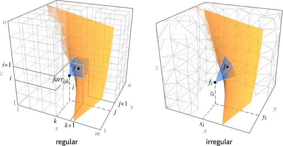
根据数组 farr 生成一个等高线图,其于点 {k,j,i} 处的值为 farr[[i,j,k]].
ListContourPlot3D[{{x1,y1,z1,f1},{x2,y2,z2,f2},…}]
根据点 {xi,yi,zi} 处的数值 fi 生成一个等高线图.
更多信息和选项
- ListContourPlot3D 也被称为等值面或水平集图.
- ListContourPlot3D 构建内插函数
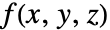 具有常数 d1, d2 等的等高线表面.
- 对于规则数据,函数
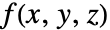 在
 处有值 farr[[i,j,k]].
- 对于不规则函数,
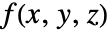 在
 处有值 fi.
- 该函数将表面
 可视化,其中区域
 为规则数据的笛卡尔积
 ,及不规则数据的 {{x1,y1,z1},…,{xn,yn,zn}} 的凸壳.
- ListContourPlot3D[Tabular[…]cspec] 使用列规范 cspec 从表格对象中提取并绘制数值.
- 下列形式的列规范 cspec 可用于绘制表格数据:
-
{colx,coly,colz,colf} 绘制 f 列与 x、y 和 z 列的对比图 - ListContourPlot3D 绘制的等高面可包含不相连的部分.
- 默认情况下,ListContourPlot3D 以不透明的白色表面显示每个等高线,法线指向外.
- ListContourPlot3D 默认情况下显示三个等高线水平,按 f 值等距离分布.
- 可选项设置为 Contours->{f0} 时,ListContourPlot3D 只显示一个等高线水平 f=f0.
- ListContourPlot3D 的可选项与 Graphics3D 一样,并具有以下补充和修改: [所有选项的列表]
-
Axes True 是否绘制坐标轴 BoundaryStyle Automatic 如何绘制区域的边界 BoxRatios {1,1,1} 3D 边界框比例 ColorFunction Automatic 如何着色等高面 ColorFunctionScaling True 是否按比例缩放 ColorFunction 的自变量 Contours 3 显示多少个等高面或哪几个等高面 ContourStyle White 等高面的样式 DataRange Automatic 对数据假设所采用的坐标值的范围 MaxPlotPoints Automatic 包含点的最大数量 Mesh Automatic 每个方向中绘制网格线的数量 MeshFunctions {#1&,#2&,#3&} 如何确定网格线的布置 MeshShading None 如何对网格线之间的区域使用阴影 MeshStyle Automatic 网格线区域的样式 Method Automatic 对插补和数据化简使用的方法 PerformanceGoal $PerformanceGoal 尝试优化的性能 PlotLegends None 曲面的图例 PlotRange {Full,Full,Full,Automatic} 包含的值范围 PlotTheme $PlotTheme 图线的整体主题 RegionFunction (True&) 如何确定是否应包含一个点 ScalingFunctions None 如何缩放单个坐标 TextureCoordinateFunction Automatic 如何确定纹理坐标 TextureCoordinateScaling True 如何对 TextureCoordinateFunction 的自变量进行尺度调整 - ListContourPlot3D 线性插补值,得出平滑的等高线.
- array 应为实数组成的的矩形数组;有非实数元素时,应在图形中留有空间.
- ListContourPlot3D[array] 在默认情况下对每个数据点采用 x、y 和 z 坐标值,数据点为从 1 开始的连续整数.
- 设置 DataRange->{{xmin,xmax},{ymin,ymax},{zmin,zmax}} 指定了使用的其它坐标值范围.
- array 可以是一个 SparseArray 对象.
- 提供给 MeshFunctions 和 RegionFunction 中函数的自变量为 x、y、z、f. ColorFunction 和 TextureCoordinateFunction 中的函数在默认情况下采用这些自变量的尺寸缩放版.
- ScalingFunctions 的可能设置包括:
-
{sx,sy,sz} 缩放 x、y 和 z 轴 - 常见的内置缩放函数 s 包括:
-
"Log" 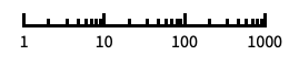
带自动刻度线的对数尺度 "Log10" 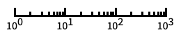
以 10 为基数的对数尺度,刻度为10的幂 "SignedLog" 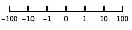
包括 0 和负数的类对数尺度 "Reverse" 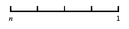
倒转坐标方向 - ListContourPlot3D 返回 Graphics3D[GraphicsComplex[data]].
- 影响三维表面的主题包括:
-
"DarkMesh" 深色的网格线 
"GrayMesh" 灰色的网格线 
"LightMesh" 浅色的网格线 
"ZMesh" 垂直分布的网格线 
"ThickSurface" 在表面添加厚度
所有选项的列表
范例
打开所有单元 关闭所有单元基本范例 (5)
ListContourPlot3D[Table[x ^ 2 + y ^ 2 - z ^ 2 + RandomReal[0.1], {x, -2, 2, 0.2}, {y, -2, 2, 0.2}, {z, -2, 2, 0.2}], Contours -> {0}, Mesh -> None]ListContourPlot3D[Table[x ^ 2 + y ^ 2 - z ^ 2 + RandomReal[0.1], {x, -2, 2, 0.2}, {y, -2, 2, 0.2}, {z, -2, 2, 0.2}], Contours -> 3, Mesh -> None]data = Table[{x = RandomReal[{-1, 1}], y = RandomReal[{-1, 1}], z = RandomReal[{-1, 1}], x ^ 2 + y ^ 2 - z ^ 2}, {5000}];ListContourPlot3D[data, Contours -> {0.5}, Mesh -> None]ListContourPlot3D[Table[x ^ 2 + y ^ 2 - z ^ 2 + RandomReal[0.1], {x, -2, 2, 0.2}, {y, -2, 2, 0.2}, {z, -2, 2, 0.2}], Contours -> 3, Mesh -> None, ContourStyle -> {Red, Orange, Yellow}]ListContourPlot3D[Table[x ^ 2 + y ^ 2 - z ^ 2, {x, -2, 2, 0.2}, {y, -2, 2, 0.2}, {z, -2, 2, 0.2}], Contours -> 5, Mesh -> None, PlotLegends -> "Expressions"]范围 (7)
数据 (5)


ListContourPlot3D[Table[Sqrt[x ^ 2 + y ^ 2 + z ^ 2], {x, 0, 3, 0.1}, {y, 0, 3, 0.1}, {z, 0, 3, 0.1}]]通过使用 DataRange,提供显式  、
 和
 数据范围:
ListContourPlot3D[Table[Sqrt[x ^ 2 + y ^ 2 + z ^ 2], {x, 0, 3, 0.1}, {y, 0, 3, 0.1}, {z, 0, 3, 0.1}], DataRange -> {{0, 3}, {0, 3}, {0, 3}}]对于包含 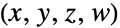 三元组的不规则数据,从数据推导
 、
 和
 数据范围:
data = Table[{x = RandomReal[{-1, 1}], y = RandomReal[{0, 1}], z = RandomReal[{-1, 1}], Sqrt[x ^ 2 + y ^ 2 + z ^ 2]}, {1000}];ListContourPlot3D[data, Mesh -> All]使用 MaxPlotPoints 限制使用的点数:
Table[ListContourPlot3D[Table[Sqrt[x ^ 2 + y ^ 2 + z ^ 2], {x, 0, 3, 0.1}, {y, 0, 3, 0.1}, {z, 0, 3, 0.1}], MaxPlotPoints -> mp, Mesh -> All], {mp, {Infinity, 15, 5}}]data = Table[{Quantity[x = RandomReal[{-1, 1}], "Meters"], Quantity[y = RandomReal[{-1, 1}], "Seconds"], Quantity[z = RandomReal[{-1, 1}], "Kilograms"], x ^ 2 + y ^ 2 - z ^ 2}, {1000}];ListContourPlot3D[data, BoxRatios -> Automatic, Contours -> {0}, AxesLabel -> Automatic]ListContourPlot3D[data, AxesLabel -> Automatic, Contours -> {0}, TargetUnits -> {"Feet", "Seconds", "Pounds", Automatic}]表格数据 (1)
选项 (93)
Axes (3)
默认情况下,ListContourPlot3D 会在图中绘制 Axes:
ListContourPlot3D[Table[Sqrt[x ^ 2 + y ^ 2 + z ^ 2], {x, 0, 3, 0.1}, {y, 0, 3, 0.1}, {z, 0, 3, 0.1}]]ListContourPlot3D[Table[Sqrt[x ^ 2 + y ^ 2 + z ^ 2], {x, 0, 3, 0.1}, {y, 0, 3, 0.1}, {z, 0, 3, 0.1}], Axes -> False]{ListContourPlot3D[Table[Sqrt[x ^ 2 + y ^ 2 + z ^ 2], {x, 0, 3, 0.1}, {y, 0, 3, 0.1}, {z, 0, 3, 0.1}], Axes -> {True, False, False}], ListContourPlot3D[Table[Sqrt[x ^ 2 + y ^ 2 + z ^ 2], {x, 0, 3, 0.1}, {y, 0, 3, 0.1}, {z, 0, 3, 0.1}], Axes -> {False, True, False}], ListContourPlot3D[Table[Sqrt[x ^ 2 + y ^ 2 + z ^ 2], {x, 0, 3, 0.1}, {y, 0, 3, 0.1}, {z, 0, 3, 0.1}], Axes -> {False, False, True}]}AxesLabel (4)
ListContourPlot3D[Table[x ^ 2 + y ^ 2 + z ^ 2, {z, -1, 1, 0.02}, {y, -1, 1, 0.02}, {x, -1, 1, 0.02}]]
ListContourPlot3D[Table[x ^ 2 + y ^ 2 + z ^ 2, {z, -1, 1, 0.02}, {y, -1, 1, 0.02}, {x, -1, 1, 0.02}], AxesLabel -> z]ListContourPlot3D[Table[x ^ 2 + y ^ 2 + z ^ 2, {z, -1, 1, 0.02}, {y, -1, 1, 0.02}, {x, -1, 1, 0.02}], AxesLabel -> {"x", "y", "z"}]data = Table[{Quantity[x = RandomReal[{-1, 1}], "Meters"], Quantity[y = RandomReal[{-1, 1}], "Seconds"], Quantity[z = RandomReal[{-1, 1}], "Kilograms"], x ^ 2 + y ^ 2 - z ^ 2}, {1000}];ListContourPlot3D[data, BoxRatios -> Automatic, Contours -> {0}, AxesLabel -> Automatic]AxesOrigin (2)
ListContourPlot3D[Table[x ^ 2 + y ^ 2 + z ^ 2, {z, -1, 1, 0.02}, {y, -1, 1, 0.02}, {x, -1, 1, 0.02}]]ListContourPlot3D[Table[x ^ 2 + y ^ 2 + z ^ 2, {z, -1, 1, 0.02}, {y, -1, 1, 0.02}, {x, -1, 1, 0.02}], AxesOrigin -> {100, 0, 100}]AxesStyle (4)
ListContourPlot3D[Table[Sqrt[x ^ 2 + y ^ 2 + z ^ 2], {x, 0, 3, 0.1}, {y, 0, 3, 0.1}, {z, 0, 3, 0.1}], AxesStyle -> Red]ListContourPlot3D[Table[Sqrt[x ^ 2 + y ^ 2 + z ^ 2], {x, 0, 3, 0.1}, {y, 0, 3, 0.1}, {z, 0, 3, 0.1}], AxesStyle -> {{Thick, Brown}, {Thick, Blue}, {Thick, Green}}]ListContourPlot3D[Table[Sqrt[x ^ 2 + y ^ 2 + z ^ 2], {x, 0, 3, 0.1}, {y, 0, 3, 0.1}, {z, 0, 3, 0.1}], AxesStyle -> Green, TicksStyle -> Red]ListContourPlot3D[Table[Sqrt[x ^ 2 + y ^ 2 + z ^ 2], {x, 0, 3, 0.1}, {y, 0, 3, 0.1}, {z, 0, 3, 0.1}], AxesStyle -> Green, LabelStyle -> Red]BoundaryStyle (3)
ListContourPlot3D[Table[Sqrt[x ^ 2 + y ^ 2 + z ^ 2], {x, 0, 3, 0.1}, {y, 0, 3, 0.1}, {z, 0, 3, 0.1}], BoundaryStyle -> Red, Mesh -> None]使用 None 忽略边界:
ListContourPlot3D[Table[Sqrt[x ^ 2 + y ^ 2 + z ^ 2], {x, 0, 3, 0.1}, {y, 0, 3, 0.1}, {z, 0, 3, 0.1}], BoundaryStyle -> None, Mesh -> None]BoundaryStyle 应用于由 RegionFunction 切割的洞:
ListContourPlot3D[Table[Sqrt[x ^ 2 + y ^ 2 + z ^ 2], {x, -3, 3, 0.1}, {y, -3, 3, 0.1}, {z, -3, 3, 0.1}], DataRange -> {{-3, 3}, {-3, 3}, {-3, 3}}, BoundaryStyle -> Red, Mesh -> None, RegionFunction -> Function[{x, y, z, w}, x < 0 || y > 0]]BoxRatios (3)
ListContourPlot3D[Table[{x = RandomReal[{-1, 1}], y = RandomReal[{-2, 2}], z = RandomReal[{-0.5, 0.5}], x ^ 2 + (y / 2) ^ 2 + (2z) ^ 2}, {2500}]]ListContourPlot3D[Table[{x = RandomReal[{-1, 1}], y = RandomReal[{-2, 2}], z = RandomReal[{-0.5, 0.5}], x ^ 2 + (y / 2) ^ 2 + (2z) ^ 2}, {2500}], BoxRatios -> {1, 2, 1 / 2}]ListContourPlot3D[Table[{x = RandomReal[{-1, 1}], y = RandomReal[{-2, 2}], z = RandomReal[{-0.5, 0.5}], x ^ 2 + (y / 2) ^ 2 + (2z) ^ 2}, {2500}], BoxRatios -> Automatic]ColorFunction (5)


Table[ListContourPlot3D[Table[x ^ 2 + y ^ 2 + z ^ 2, {x, -3, 3, 0.1}, {y, -3, 3, 0.1}, {z, -3, 3, 0.1}], ColorFunction -> Function[{x, y, z, f}, Evaluate[c]], PlotLabel -> c, Axes -> None], {c, {Hue[x], Hue[y], Hue[z], Hue[f]}}]ListContourPlot3D[Table[x ^ 2 + y ^ 2 + z ^ 2, {x, -3, 3, 0.1}, {y, -3, 3, 0.1}, {z, -3, 3, 0.1}], Mesh -> None, Contours -> 4, ColorFunction -> "DarkRainbow"]ColorFunction 具有比 ContourStyle 更高的优先级:
ListContourPlot3D[Table[x ^ 2 + y ^ 2 + z ^ 2, {x, -3, 3, 0.1}, {y, -3, 3, 0.1}, {z, -3, 3, 0.1}], Mesh -> None, Contours -> 4, ColorFunction -> "DarkRainbow", ContourStyle -> Directive[Opacity[0.5], Red]]
ListContourPlot3D[Table[x ^ 2 + y ^ 2 + z ^ 2, {x, -3, 3, 0.1}, {y, -3, 3, 0.1}, {z, -3, 3, 0.1}], DataRange -> {{-3, 3}, {-3, 3}, {-3, 3}}, ColorFunction -> Function[{x, y, z, f}, If[z < 0, Red, Green]], ColorFunctionScaling -> False]ColorFunction 具有比 MeshShading 更低的优先级:
ListContourPlot3D[Table[x ^ 2 + y ^ 2 + z ^ 2, {x, -3, 3, 0.1}, {y, -3, 3, 0.1}, {z, -3, 3, 0.1}], ColorFunction -> Function[{x, y, z, f}, Hue[z]], MeshFunctions -> {#3&}, MeshShading -> {Automatic, StandardGray}]ColorFunctionScaling (2)
ListContourPlot3D[Table[x ^ 2 + y ^ 2 + z ^ 2, {x, -3, 3, 0.1}, {y, -3, 3, 0.1}, {z, -3, 3, 0.1}], Mesh -> None, Contours -> 4, ColorFunction -> Function[{x, y, z, f}, Hue[f / 5]], ColorFunctionScaling -> False]ListContourPlot3D[Table[x ^ 2 + y ^ 2 + z ^ 2, {x, -3, 3, 0.1}, {y, -3, 3, 0.1}, {z, -3, 3, 0.1}], DataRange -> {{-3, 3}, {-3, 3}, {-3, 3}}, ColorFunction -> Function[{x, y, z, f}, Hue[Sin[x]Sin[y]]], ColorFunctionScaling -> False, Mesh -> None]Contours (3)
ListContourPlot3D[Table[x ^ 3 + y ^ 2 - z ^ 2, {z, -2, 2, 0.1}, {y, -2, 2, 0.1}, {x, -2, 2, 0.1}], Contours -> 5, Mesh -> None]ListContourPlot3D[Table[x ^ 3 + y ^ 2 - z ^ 2, {z, -2, 2, 0.1}, {y, -2, 2, 0.1}, {x, -2, 2, 0.1}], Contours -> Automatic, Mesh -> None]ListContourPlot3D[Table[x ^ 3 + y ^ 2 - z ^ 2, {z, -2, 2, 0.1}, {y, -2, 2, 0.1}, {x, -2, 2, 0.1}], Contours -> {-2, 2}, Mesh -> None]ContourStyle (7)
ListContourPlot3D[Table[x ^ 2 + y ^ 2 + z ^ 2, {z, -2, 2, 0.1}, {y, -2, 2, 0.1}, {x, -2, 2, 0.1}], Mesh -> None, ContourStyle -> Opacity[0.5]]ListContourPlot3D[Table[x ^ 2 + y ^ 2 + z ^ 2, {z, -2, 2, 0.1}, {y, -2, 2, 0.1}, {x, -2, 2, 0.1}], Mesh -> None, ContourStyle -> {Red, Green, Blue}]使用 FaceForm 以获取内在和外在的不同颜色:
ListContourPlot3D[Table[x ^ 2 + y ^ 2 - z ^ 2, {z, -2, 2, 0.1}, {y, -2, 2, 0.1}, {x, -2, 2, 0.1}], Contours -> {1}, Mesh -> 5, ContourStyle -> {FaceForm[Yellow, Blue]}]ListContourPlot3D[Table[x ^ 2 + y ^ 2 + z ^ 2, {z, -2, 2, 0.1}, {y, -2, 2, 0.1}, {x, -2, 2, 0.1}], Contours -> 4, Mesh -> None, ContourStyle -> {Blue, Opacity[0.5]}]ListContourPlot3D[Table[x ^ 2 + y ^ 2 + z ^ 2, {z, -2, 2, 0.1}, {y, -2, 2, 0.1}, {x, -2, 2, 0.1}], Contours -> 6, Mesh -> None, ContourStyle -> Directive[Opacity[0.5], Orange]]ColorFunction 具有比 ContourStyle 更高的优先级:
ListContourPlot3D[Table[x ^ 2 + y ^ 2 - z ^ 2, {z, -2, 2, 0.1}, {y, -2, 2, 0.1}, {x, -2, 2, 0.1}], Contours -> {1}, Mesh -> None, ContourStyle -> Directive[Opacity[0.5], Red], ColorFunction -> Function[{x, y, z, f}, Hue[z]]]MeshShading 具有比 ContourStyle 更高的优先级:
ListContourPlot3D[Table[x ^ 2 + y ^ 2 - z ^ 2, {z, -2, 2, 0.1}, {y, -2, 2, 0.1}, {x, -2, 2, 0.1}], Contours -> {1}, MeshFunctions -> {#3&}, ContourStyle -> Directive[Opacity[0.5], Yellow], MeshShading -> {Red, Automatic}]DataRange (3)
ListContourPlot3D[Table[x ^ 3 + y ^ 2 - z ^ 2, {z, -2, 2, 0.1}, {y, -2, 2, 0.1}, {x, -2, 2, 0.1}]]ListContourPlot3D[Table[x ^ 3 + y ^ 2 - z ^ 2, {z, -2, 2, 0.1}, {y, -2, 2, 0.1}, {x, -2, 2, 0.1}], DataRange -> {{-2, 2}, {-2, 2}, {-2, 2}}]


data = Table[{x = RandomReal[{-2, 2}], y = RandomReal[{-2, 2}], z = RandomReal[{-2, 2}], x ^ 3 + y ^ 2 - z ^ 2}, {2500}];ListContourPlot3D[data]ImageSize (7)
使用已命名尺寸,如 Tiny、Small、Medium 和 Large:
{ListContourPlot3D[Table[Sqrt[x ^ 2 + y ^ 2 + z ^ 2], {x, 0, 3, 0.1}, {y, 0, 3, 0.1}, {z, 0, 3, 0.1}], ImageSize -> Tiny], ListContourPlot3D[Table[Sqrt[x ^ 2 + y ^ 2 + z ^ 2], {x, 0, 3, 0.1}, {y, 0, 3, 0.1}, {z, 0, 3, 0.1}], ImageSize -> Small]}{ListContourPlot3D[Table[Sqrt[x ^ 2 + y ^ 2 + z ^ 2], {x, 0, 3, 0.1}, {y, 0, 3, 0.1}, {z, 0, 3, 0.1}], ImageSize -> 150], ListContourPlot3D[Table[Sqrt[x ^ 2 + y ^ 2 + z ^ 2], {x, 0, 3, 0.1}, {y, 0, 3, 0.1}, {z, 0, 3, 0.1}], AspectRatio -> 1.5, ImageSize -> 150]}{ListContourPlot3D[Table[Sqrt[x ^ 2 + y ^ 2 + z ^ 2], {x, 0, 3, 0.1}, {y, 0, 3, 0.1}, {z, 0, 3, 0.1}], ImageSize -> {Automatic, 150}], ListContourPlot3D[Table[Sqrt[x ^ 2 + y ^ 2 + z ^ 2], {x, 0, 3, 0.1}, {y, 0, 3, 0.1}, {z, 0, 3, 0.1}], AspectRatio -> 2, ImageSize -> {Automatic, 150}]}{ListContourPlot3D[Table[Sqrt[x ^ 2 + y ^ 2 + z ^ 2], {x, 0, 3, 0.1}, {y, 0, 3, 0.1}, {z, 0, 3, 0.1}], ImageSize -> UpTo[200]], ListContourPlot3D[Table[Sqrt[x ^ 2 + y ^ 2 + z ^ 2], {x, 0, 3, 0.1}, {y, 0, 3, 0.1}, {z, 0, 3, 0.1}], AspectRatio -> 2, ImageSize -> UpTo[200]]}ListContourPlot3D[Table[Sqrt[x ^ 2 + y ^ 2 + z ^ 2], {x, 0, 3, 0.1}, {y, 0, 3, 0.1}, {z, 0, 3, 0.1}], ImageSize -> {200, 250}, Background -> StandardGray]设置 AspectRatioFull 将填充可用空间:
ListContourPlot3D[Table[Sqrt[x ^ 2 + y ^ 2 + z ^ 2], {x, 0, 3, 0.1}, {y, 0, 3, 0.1}, {z, 0, 3, 0.1}], AspectRatio -> Full, ImageSize -> {200, 250}, Background -> StandardGray]{ListContourPlot3D[Table[Sqrt[x ^ 2 + y ^ 2 + z ^ 2], {x, 0, 3, 0.1}, {y, 0, 3, 0.1}, {z, 0, 3, 0.1}], ImageSize -> {UpTo[150], UpTo[150]}], ListContourPlot3D[Table[Sqrt[x ^ 2 + y ^ 2 + z ^ 2], {x, 0, 3, 0.1}, {y, 0, 3, 0.1}, {z, 0, 3, 0.1}], AspectRatio -> 2, ImageSize -> {UpTo[150], UpTo[150]}]}Framed[Pane[ListContourPlot3D[Table[Sqrt[x ^ 2 + y ^ 2 + z ^ 2], {x, 0, 3, 0.1}, {y, 0, 3, 0.1}, {z, 0, 3, 0.1}], ImageSize -> Full, Background -> StandardGray], {200, 100}]]Framed[Pane[ListContourPlot3D[Table[Sqrt[x ^ 2 + y ^ 2 + z ^ 2], {x, 0, 3, 0.1}, {y, 0, 3, 0.1}, {z, 0, 3, 0.1}], AspectRatio -> Full, ImageSize -> {Scaled[0.5], Scaled[0.5]}, Background -> StandardGray], {200, 200}]]MaxPlotPoints (3)
ListContourPlot 通常使用数据集中所有点:
ListContourPlot3D[Table[x ^ 3 + y ^ 2 - z ^ 2, {z, -2, 2, 0.1}, {y, -2, 2, 0.1}, {x, -2, 2, 0.1}], Mesh -> All]data = Table[{x = RandomReal[{-2, 2}], y = RandomReal[{-2, 2}], z = RandomReal[{-2, 2}], x ^ 3 + y ^ 2 - z ^ 2}, {5000}];ListContourPlot3D[data, Mesh -> All]ListContourPlot3D[Table[x ^ 3 + y ^ 2 - z ^ 2, {z, -2, 2, 0.1}, {y, -2, 2, 0.1}, {x, -2, 2, 0.1}], MaxPlotPoints -> 10, Mesh -> All]MaxPlotPoints 在不规则数据上强加规则网格:
data = Table[{x = RandomReal[{-2, 2}], y = RandomReal[{-2, 2}], z = RandomReal[{-2, 2}], x ^ 3 + y ^ 2 - z ^ 2}, {5000}];ListContourPlot3D[data, MaxPlotPoints -> 10, Mesh -> All]Mesh (6)
ListContourPlot3D[Table[x ^ 3 + y ^ 2 - z ^ 2, {z, -2, 2, 0.1}, {y, -2, 2, 0.1}, {x, -2, 2, 0.1}], Mesh -> All]使用 None 不绘制任何网格:
ListContourPlot3D[Table[x ^ 3 + y ^ 2 - z ^ 2, {z, -2, 2, 0.1}, {y, -2, 2, 0.1}, {x, -2, 2, 0.1}], Mesh -> None]ListContourPlot3D[Table[x ^ 3 + y ^ 2 - z ^ 2, {z, -2, 2, 0.1}, {y, -2, 2, 0.1}, {x, -2, 2, 0.1}], Mesh -> 5, MeshFunctions -> {#1&, #2&, #3&}]

ListContourPlot3D[Table[x ^ 3 + y ^ 2 - z ^ 2, {z, -2, 2, 0.1}, {y, -2, 2, 0.1}, {x, -2, 2, 0.1}], Mesh -> {5, 10}, MeshFunctions -> {#1&, #2&}]ListContourPlot3D[Table[x ^ 2 + y ^ 2 + z ^ 2, {z, -2, 2, 0.1}, {y, -2, 2, 0.1}, {x, -2, 2, 0.1}], DataRange -> {{-2, 2}, {-2, 2}, {-2, 2}}, Contours -> {1}, Mesh -> {{0}, {0}}, MeshFunctions -> {#1&, #2&}]ListContourPlot3D[Table[x ^ 2 + y ^ 2 + z ^ 2, {z, -2, 2, 0.1}, {y, -2, 2, 0.1}, {x, -2, 2, 0.1}], DataRange -> {{-2, 2}, {-2, 2}, {-2, 2}}, Contours -> {1}, Mesh -> {{{0, Thick}}, {{0, Red}}}]MeshFunctions (2)


Table[ListContourPlot3D[Table[x ^ 2 + y ^ 2 + z ^ 2, {z, -2, 2, 0.1}, {y, -2, 2, 0.1}, {x, -2, 2, 0.1}], DataRange -> {{-2, 2}, {-2, 2}, {-2, 2}}, Contours -> {1}, PlotLabel -> f, MeshFunctions -> {Function[{x, y, z}, f]}, Axes -> None], {f, {x, y, z}}]ListContourPlot3D[Table[x ^ 3 + y ^ 2 - z ^ 2, {z, -2, 2, 0.1}, {y, -2, 2, 0.1}, {x, -2, 2, 0.1}], DataRange -> {{-2, 2}, {-2, 2}, {-2, 2}}, MeshFunctions -> (Norm[{#1, #2, #3}]&)]MeshShading (5)

ListContourPlot3D[Table[x ^ 2 + y ^ 2 - z ^ 2, {z, -2, 2, 0.1}, {y, -2, 2, 0.1}, {x, -2, 2, 0.1}], Contours -> {1}, MeshFunctions -> {#3&}, MeshShading -> {Red, Blue}]在样式配置上,MeshShading 比 ContourStyle 的优先级高:
ListContourPlot3D[Table[x ^ 2 + y ^ 2 - z ^ 2, {z, -2, 2, 0.1}, {y, -2, 2, 0.1}, {x, -2, 2, 0.1}], Contours -> 1, MeshFunctions -> {#3&}, MeshShading -> {None, Blue}]将 MeshShading 设为 Automatic,同时使用 ContourStyle 来指定某些部分的样式:
ListContourPlot3D[Table[x ^ 2 + y ^ 2 - z ^ 2, {z, -2, 2, 0.1}, {y, -2, 2, 0.1}, {x, -2, 2, 0.1}], Contours -> {1}, MeshFunctions -> {#3&}, MeshShading -> {Red, Automatic}, ContourStyle -> Directive[Opacity[0.5], Yellow]]MeshShading 可与 ColorFunction 一起使用:
ListContourPlot3D[Table[x ^ 2 + y ^ 2 - z ^ 2, {z, -2, 2, 0.1}, {y, -2, 2, 0.1}, {x, -2, 2, 0.1}], Contours -> {1}, MeshFunctions -> {#3&}, MeshShading -> {StandardGray, Automatic}, ColorFunction -> Function[{x, y, z, f}, Hue[z]]]ListContourPlot3D[Table[x ^ 2 + y ^ 2 - z ^ 2, {z, -2, 2, 0.1}, {y, -2, 2, 0.1}, {x, -2, 2, 0.1}], Contours -> {1}, Mesh -> 5, Lighting -> "Neutral", MeshShading -> Table[RGBColor[r, g, b], {r, 0, 1, 1 / 5}, {g, 0, 1, 1 / 5}, {b, 0, 1, 1 / 5}]]MeshStyle (2)

ListContourPlot3D[Table[x ^ 2 + y ^ 2 - z ^ 2, {z, -2, 2, 0.1}, {y, -2, 2, 0.1}, {x, -2, 2, 0.1}], Contours -> {1}, MeshFunctions -> {#1&}, MeshStyle -> Dashed, Mesh -> 5]

ListContourPlot3D[Table[x ^ 2 + y ^ 2 - z ^ 2, {z, -2, 2, 0.1}, {y, -2, 2, 0.1}, {x, -2, 2, 0.1}], Contours -> {1}, Mesh -> 5, MeshFunctions -> {#1&, #2&}, MeshStyle -> {Dashed, Blue}]PerformanceGoal (2)
Timing[ListContourPlot3D[Table[x ^ 2 + y ^ 2 - z ^ 2, {z, -2, 2, 0.1}, {y, -2, 2, 0.1}, {x, -2, 2, 0.1}], PerformanceGoal -> "Quality"]]Timing[ListContourPlot3D[Table[x ^ 2 + y ^ 2 - z ^ 2, {z, -2, 2, 0.1}, {y, -2, 2, 0.1}, {x, -2, 2, 0.1}], PerformanceGoal -> "Speed"]]PlotRange (2)


ListContourPlot3D[Table[x ^ 2 + y ^ 2 + z ^ 2, {z, -2, 2, 0.1}, {y, -2, 2, 0.1}, {x, -2, 2, 0.1}], DataRange -> {{-2, 2}, {-2, 2}, {-2, 2}}, Contours -> 5]ListContourPlot3D[Table[x ^ 2 + y ^ 2 + z ^ 2, {z, -2, 2, 0.1}, {y, -2, 2, 0.1}, {x, -2, 2, 0.1}], DataRange -> {{-2, 2}, {-2, 2}, {-2, 2}}, Contours -> 5, PlotRange -> {{-2, 0}, {-2, 2}, {-2, 2}}, BoxRatios -> Automatic]PlotTheme (3)
ListContourPlot3D[Table[x ^ 2 + y ^ 2 - z ^ 2, {z, -2, 2, 0.1}, {y, -2, 2, 0.1}, {x, -2, 2, 0.1}], PlotTheme -> "Marketing"]ListContourPlot3D[Table[x ^ 2 + y ^ 2 - z ^ 2, {z, -2, 2, 0.1}, {y, -2, 2, 0.1}, {x, -2, 2, 0.1}], PlotTheme -> "Marketing", Ticks -> None, Mesh -> 5]ListContourPlot3D[Table[x ^ 2 + y ^ 2 - z ^ 2, {z, -2, 2, 0.1}, {y, -2, 2, 0.1}, {x, -2, 2, 0.1}], Contours -> {0}, PlotTheme -> "ThickSurface"]RegionFunction (2)


Table[ListContourPlot3D[Table[x ^ 2 + y ^ 2 + z ^ 2, {z, -1, 1, 0.02}, {y, -1, 1, 0.02}, {x, -1, 1, 0.02}], DataRange -> {{-1, 1}, {-1, 1}, {-1, 1}}, Mesh -> None, Axes -> None, Contours -> 4, RegionFunction -> Function[{x, y, z}, Evaluate[f]], PlotLabel -> f], {f, {-1 / 2 < x < 1 / 2, -1 / 2 < y < 1 / 2, -1 / 2 < z < 1 / 2}}]ListContourPlot3D[Table[x ^ 2 + y ^ 2 + z ^ 2, {z, -1, 1, 0.02}, {y, -1, 1, 0.02}, {x, -1, 1, 0.02}], DataRange -> {{-1, 1}, {-1, 1}, {-1, 1}}, Contours -> 4, Mesh -> None, Axes -> None, RegionFunction -> Function[{x, y, z}, x < 0 || y > 0]]ScalingFunctions (4)
默认情况下,ContourPlot3D 在所有的方向上都使用线性尺度:
ListContourPlot3D[Table[x ^ 2 + y ^ 2 - z, {z, 1, 10, 0.1}, {y, -2, 2, 0.1}, {x, -2, 2, 0.1}]]
ListContourPlot3D[Table[x ^ 2 + y ^ 2 - z, {z, 1, 10, 0.1}, {y, -2, 2, 0.1}, {x, -2, 2, 0.1}], ScalingFunctions -> {None, None, "Log"}, PlotRange -> All]
ListContourPlot3D[Table[x ^ 2 + y ^ 2 - z, {z, 1, 10, 0.1}, {y, -2, 2, 0.1}, {x, -2, 2, 0.1}], ScalingFunctions -> {None, None, "Reverse"}]ListContourPlot3D[Table[x ^ 2 + y ^ 2 - z, {z, 1, 10, 0.1}, {y, -2, 2, 0.1}, {x, -2, 2, 0.1}], ScalingFunctions -> {None, None, {-Log[# + 1]&, Exp[-#] - 1&}}]TargetUnits (1)
data = Table[{Quantity[x = RandomReal[{-1, 1}], "Meters"], Quantity[y = RandomReal[{-1, 1}], "Seconds"], Quantity[z = RandomReal[{-1, 1}], "Kilograms"], x ^ 2 + y ^ 2 - z ^ 2}, {1000}];ListContourPlot3D[data, BoxRatios -> Automatic, Contours -> {0}, AxesLabel -> Automatic]ListContourPlot3D[data, AxesLabel -> Automatic, Contours -> {0}, TargetUnits -> {"Feet", "Seconds", "Pounds", Automatic}]TextureCoordinateFunction (5)


ListContourPlot3D[Table[x ^ 2 + y ^ 2 - z ^ 2, {x, -2, 2, 0.1}, {y, -2, 2, 0.1}, {z, -2, 2, 0.1}], Contours -> {1}, Mesh -> None, Lighting -> "Neutral", ContourStyle -> Texture[ExampleData[{"ColorTexture", "WavesPattern"}]]]

ListContourPlot3D[Table[x ^ 2 + y ^ 2 - z ^ 2, {x, -2, 2, 0.1}, {y, -2, 2, 0.1}, {z, -2, 2, 0.1}], Contours -> {1}, Mesh -> None, Lighting -> "Neutral", TextureCoordinateFunction -> ({#1, #3}&), ContourStyle -> Texture[ExampleData[{"ColorTexture", "WavesPattern"}]]]ListContourPlot3D[Table[x ^ 2 + y ^ 2 - z ^ 2, {x, -2, 2, 0.1}, {y, -2, 2, 0.1}, {z, -2, 2, 0.1}], Mesh -> None, Lighting -> "Neutral", ContourStyle -> {Texture[ExampleData[{"ColorTexture", "Ash"}]], Texture[ExampleData[{"ColorTexture", "Amboyna"}]], Texture[ExampleData[{"ColorTexture", "Laurel"}]]}]ListContourPlot3D[Table[x ^ 2 + y ^ 2 - z ^ 2, {x, -2, 2, 0.1}, {y, -2, 2, 0.1}, {z, -2, 2, 0.1}], Contours -> {1}, Mesh -> None, Lighting -> "Neutral", TextureCoordinateScaling -> False, ContourStyle -> Texture[ExampleData[{"ColorTexture", "WavesPattern"}]]]texture = ArrayPlot[{{1, 1, 1, 2, 1, 1}, {2, 0, 0, 2, 0, 0}, {2, 0, 0, 2, 0, 0}, {2, 1, 1, 1, 1, 1}, {2, 0, 0, 2, 0, 0}, {2, 0, 0, 2, 0, 0}}, ColorRules -> {1 -> Red, 2 -> Blue, 0 -> White}, Frame -> False, PlotRangePadding -> None, ImagePadding -> None, ImageSize -> 100]ListContourPlot3D[Table[x ^ 2 + y ^ 2 - z ^ 2, {x, -2, 2, 0.1}, {y, -2, 2, 0.1}, {z, -2, 2, 0.1}], Contours -> {1}, Mesh -> None, Lighting -> "Neutral", ContourStyle -> Texture[texture]]TextureCoordinateScaling (1)
texture = ArrayPlot[{{1, 1, 1, 2, 1, 1}, {2, 0, 0, 2, 0, 0}, {2, 0, 0, 2, 0, 0}, {2, 1, 1, 1, 1, 1}, {2, 0, 0, 2, 0, 0}, {2, 0, 0, 2, 0, 0}}, ColorRules -> {1 -> Red, 2 -> Blue, 0 -> White}, Frame -> False, PlotRangePadding -> None, ImagePadding -> None, ImageSize -> 100]Table[ListContourPlot3D[Table[x ^ 2 + y ^ 2 - z ^ 2, {x, -2, 2, 0.1}, {y, -2, 2, 0.1}, {z, -2, 2, 0.1}], Mesh -> None, Lighting -> "Neutral", ContourStyle -> Texture[texture], TextureCoordinateScaling -> s, PlotLabel -> s], {s, {True, False}}]Ticks (6)
ListContourPlot3D[Table[x ^ 2 + y ^ 2 - z ^ 2, {x, -2, 2, 0.2}, {y, -2, 2, 0.2}, {z, -4, 4, .2}], Mesh -> None]ListContourPlot3D[Table[x ^ 2 + y ^ 2 - z ^ 2, {x, -2, 2, 0.2}, {y, -2, 2, 0.2}, {z, -4, 4, .2}], Mesh -> None, Ticks -> None]ListContourPlot3D[Table[x ^ 2 + y ^ 2 - z ^ 2, {x, -2, 2, 0.2}, {y, -2, 2, 0.2}, {z, -4, 4, .2}], Mesh -> None, Ticks -> {{0, 20, 40}, {0, 10, 20}, {0, 10, 20}}]ListContourPlot3D[Table[x ^ 2 + y ^ 2 - z ^ 2, {x, -2, 2, 0.2}, {y, -2, 2, 0.2}, {z, -4, 4, .2}], Mesh -> None, Ticks -> {{{0, a}, {20, b}, {40, c}}, {{0, a}, {10, b / 2}, {20, b}}, {{0, a}, {10, b / 2}, {20, b}}}]ListContourPlot3D[Table[x ^ 2 + y ^ 2 - z ^ 2, {x, -2, 2, 0.2}, {y, -2, 2, 0.2}, {z, -4, 4, .2}], Mesh -> None, Ticks -> {{{0, a, .05}, {20, b, .17}, {40, c, .09}}, {{0, a, .01}, {10, b / 2, .05}, {20, b, .01}}, {{0, a, .01}, {10, b / 2, .08}, {20, b, .02}}}]ListContourPlot3D[Table[x ^ 2 + y ^ 2 - z ^ 2, {x, -2, 2, 0.2}, {y, -2, 2, 0.2}, {z, -4, 4, .2}], Mesh -> None, Ticks -> {{{0, a, .05, Directive[Thick, Red]}, {20, b, .17, Directive[Thick, Red]}, {40, c, .09, Directive[Thick, Red]}}, {{0, a, .01, Directive[Thick, Blue]}, {10, b / 2, .03, Directive[Thick, Blue]}, {20, b, .01, Directive[Thick, Blue]}}, {{0, a, .01, Directive[Thick, Green]}, {10, b / 2, .08, Directive[Thick, Green]}, {20, b, .02, Directive[Thick, Green]}}}]TicksStyle (3)
ListContourPlot3D[Table[x ^ 2 + y ^ 2 - z ^ 2, {x, -2, 2, 0.2}, {y, -2, 2, 0.2}, {z, -4, 4, .2}], Mesh -> None, AxesStyle -> Directive[Red, Thick]]ListContourPlot3D[Table[x ^ 2 + y ^ 2 - z ^ 2, {x, -2, 2, 0.2}, {y, -2, 2, 0.2}, {z, -4, 4, .2}], Mesh -> None, TicksStyle -> Red]ListContourPlot3D[Table[x ^ 2 + y ^ 2 - z ^ 2, {x, -2, 2, 0.2}, {y, -2, 2, 0.2}, {z, -4, 4, .2}], Mesh -> None, TicksStyle -> {Red, Directive[Blue, Bold], Directive[Brown, 16]}]文本
Wolfram Research (2007),ListContourPlot3D,Wolfram 语言函数,https://reference.wolfram.com/language/ref/ListContourPlot3D.html (更新于 2025 年).
CMS
Wolfram 语言. 2007. "ListContourPlot3D." Wolfram 语言与系统参考资料中心. Wolfram Research. 最新版本 2025. https://reference.wolfram.com/language/ref/ListContourPlot3D.html.
APA
Wolfram 语言. (2007). ListContourPlot3D. Wolfram 语言与系统参考资料中心. 追溯自 https://reference.wolfram.com/language/ref/ListContourPlot3D.html 年