


NMaxValue
NMaxValue[f,x]
gives the global maximum value of f with respect to x.
NMaxValue[f,{x,y,…}]
gives the global maximum value of f with respect to x, y, ….
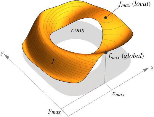
NMaxValue[{f,cons},{x,y,…}]
gives the global maximum value of f subject to the constraints cons.
NMaxValue[…,x∈reg]
constrains x to be in the region reg.
Details and Options
- NMaxValue is also known as global optimization (GO).
- NMaxValue always attempts to find a global maximum of f subject to the constraints given.
- NMaxValue is typically used to find the largest possible values given constraints. In different areas, this may be called the best strategy, best fit, best configuration and so on.
- If f is linear or concave and cons are linear or convex, the result given by NMaxValue will be the global maximum, over both real and integer values; otherwise, the result may sometimes only be a local maximum.
- If NMaxValue determines that the constraints cannot be satisfied, it returns -Infinity.
- NMaxValue supports a modeling language where the objective function f and constraints cons are given in terms of expressions depending on scalar or vector variables. f and cons are typically parsed into very efficient forms, but as long as f and the terms in cons give numerical values for numerical values of the variables, NMaxValue can often find a solution.
- The constraints cons can be any logical combination of:
-
lhs==rhs equations lhs>rhs, lhs≥rhs, lhs<rhs, lhs≤rhs inequalities (LessEqual, …) lhsrhs, lhsrhs, lhsrhs, lhsrhs vector inequalities (VectorLessEqual, …) {x,y,…}∈rdom region or domain specification - NMaxValue[{f,cons},x∈rdom] is effectively equivalent to NMaxValue[{f,cons&&x∈rdom},x].
- For x∈rdom, the different coordinates can be referred to using Indexed[x,i].
- Possible domains rdom include:
-
Reals real scalar variable Integers integer scalar variable Vectors[n,dom] vector variable in 
Matrices[{m,n},dom] matrix variable in 
ℛ vector variable restricted to the geometric region 
- By default, all variables are assumed to be real.
- The following options can be given:
-
AccuracyGoal Automatic number of digits of final accuracy sought EvaluationMonitor None expression to evaluate whenever f is evaluated MaxIterations Automatic maximum number of iterations to use Method Automatic method to use PrecisionGoal Automatic number of digits of final precision sought StepMonitor None expression to evaluate whenever a step is taken WorkingPrecision MachinePrecision the precision used in internal computations - The settings for AccuracyGoal and PrecisionGoal specify the number of digits to seek in both the value of the position of the maximum, and the value of the function at the maximum.
- NMaxValue continues until either of the goals specified by AccuracyGoal or PrecisionGoal is achieved.
- The methods for NMaxValue fall into two classes. The first class of guaranteed methods uses properties of the problem so that, when the method converges, the maximum found is guaranteed to be global. The second class of heuristic methods uses methods that may include multiple local searches, commonly adjusted by some stochasticity, to home in on a global maximum. These methods often do find the global maximum, but are not guaranteed to do so.
- Methods that are guaranteed to give a global maximum when they converge to a solution include:
-
"Convex" use only convex methods "MOSEK" use the commercial MOSEK library for convex problems "Gurobi" use the commercial Gurobi library for convex problems "Xpress" use the commercial Xpress library for convex problems - Heuristic methods include:
-
"NelderMead" simplex method of Nelder and Mead "DifferentialEvolution" use differential evolution "SimulatedAnnealing" use simulated annealing "RandomSearch" use the best local minimum found from multiple random starting points "Couenne" use the Couenne library for non-convex mixed-integer nonlinear problems
Examples
open all close allBasic Examples (5)
Find the global maximum value of a univariate function:
NMaxValue[-2x ^ 2 - 3x + 5, x]Find the global maximum value of a multivariate function:
NMaxValue[1 - (x y - 3) ^ 2, {x, y}]Find the global maximum value of a function subject to constraints:
NMaxValue[{x - 2y, x ^ 2 + y ^ 2 ≤ 1}, {x, y}]Find the global maximum value of a function over a geometric region:
MaxValue[x + y, {x, y}∈Disk[]]Find the global maximum value of a function over a geometric region:
NMaxValue[x + y, {x, y}∈Disk[]]Scope (34)
Basic Uses (12)
Maximize ![]() subject to constraints
subject to constraints ![]() :
:
NMaxValue[{x + 2y, x^2 + 2y^2 ≤ 3, x + y == 2, x ≥ 1}, {x, y}]Several linear inequality constraints can be expressed with VectorGreaterEqual:
NMaxValue[{-x - y, VectorGreaterEqual[{{x + 2y, x}, {3, -1}}]}, {x, y}]Use ![]() v>=
v>=![]() or \[VectorGreaterEqual] to enter the vector inequality sign :
or \[VectorGreaterEqual] to enter the vector inequality sign :
NMaxValue[{-x - y, {x + 2y, x}{3, -1}}, {x, y}]An equivalent form using scalar inequalities:
NMaxValue[{-x - y, x + 2y ≥ 3, x ≥ -1}, {x, y}]NMaxValue[{{-1, -1}.v, {{1, 2}, {1, 0}}.v{3, -1}}, v]The inequality ![]() may not be the same as
may not be the same as ![]() due to possible threading in
due to possible threading in ![]() :
:
NMaxValue[{{-1, -1}.x, {{1, 2}, {1, 0}}.x + {-3, 1}0}, x]NMaxValue[{{-1, -1}.x, {{1, 2}, {1, 0}}.x{3, -1}}, x]To avoid unintended threading in ![]() , use Inactive[Plus]:
, use Inactive[Plus]:
NMaxValue[{{-1, -1}.x, {{1, 2}, {1, 0}}.x + {-3, 1}0}, x]Use constant parameter equations to avoid unintended threading in ![]() :
:
parEqs = {a == {{1, 2}, {1, 0}}, b == {3, -1}};NMaxValue[{{-1, -1}.x, {parEqs, a.x + b0}}, x]VectorGreaterEqual represents a conic inequality with respect to the "NonNegativeCone":
constraint = VectorGreaterEqual[{{{1, 2}, {1, 0}}.v, {3, -1}}, "NonNegativeCone"]To explicitly specify the dimension of the cone, use {"NonNegativeCone",n}:
constraint = VectorGreaterEqual[{{{1, 2}, {1, 0}}.v, {3, -1}}, {"NonNegativeCone", 2}]NMaxValue[{{-1, -1}.v, constraint}, v]Maximize ![]() subject to the constraint
subject to the constraint ![]() :
:
NMaxValue[{x + 2y, x^2 + y^2 ≤ 9}, {x, y}]Specify the constraint ![]() using a conic inequality with "NormCone":
using a conic inequality with "NormCone":
constraint = VectorGreaterEqual[{{x, y, 3}, 0}, {"NormCone", 3}]NMaxValue[{x + 2y, constraint}, {x, y}]Maximize the function ![]() subject to the constraint
subject to the constraint ![]() :
:
{a, b} = {-{{1, 1, 0}, {0, 1, 1}, {1, 1, 1}}, {2, 2, -1}};Use Indexed to access components of a vector variable, e.g. ![]() :
:
NMaxValue[{Total[x], a.xb, Indexed[x, 1] ≥ 1}, x]Use Vectors[n,dom] to specify the dimension and domain of a vector variable when it is ambiguous:
NMaxValue[{Indexed[x, {1}] + 2Indexed[x, {2}], (| | |
| ---------------- | ---------------- |
| Indexed[-x, {1}] | 1 |
| 1 | Indexed[-x, {2}] |)Underscript[, {"SemidefiniteCone", 2}]0}, x]NMaxValue[{Indexed[x, {1}] + Indexed[2x, {2}], (| | |
| ---------------- | ---------------- |
| Indexed[-x, {1}] | 1 |
| 1 | Indexed[-x, {2}] |)Underscript[, {"SemidefiniteCone", 2}]0}, x∈Vectors[2, Reals]]Specify non-negative constraints using NonNegativeReals (![]() ):
):
NMaxValue[{{1, 1}.x, {Indexed[x, {1}], Indexed[x, {2}], 1}Underscript[, {"NormCone", 3}]0}, x∈Vectors[2, NonNegativeReals]]An equivalent form using vector inequality ![]() :
:
NMaxValue[{{1, 1}.x, {Indexed[x, {1}], Indexed[x, {2}], 1}Underscript[, {"NormCone", 3}]0, x0}, x]Specify non-positive constraints using NonPositiveReals (![]() ):
):
NMaxValue[{Total[v], {1, 2}.v-3}, v∈Vectors[2, NonPositiveReals]]An equivalent form using vector inequalities:
NMaxValue[{Total[v], {1, 2}.v-3, v0}, v]Or constraints can be specified:
NMaxValue[{x + y, x ^ 2 + y ^ 2 ≤ 1 || (x + 2) ^ 2 + (y + 2) ^ 2 ≤ 1}, {x, y}]//QuietDomain Constraints (4)
Specify integer domain constraints using Integers:
NMaxValue[{x + y, x + 2y ≤ 3, x ≤ 1}, {x, y∈Integers}]Specify integer domain constraints on vector variables using Vectors[n,Integers]:
NMaxValue[{Total[x], a == {{1, 2}, {1, 0}}, b == {-3, 2},
a.xb}, x∈Vectors[2, Integers]]Specify non-negative integer domain constraints using NonNegativeIntegers (![]() ):
):
NMaxValue[{x + 2y, x^2 + 2y^2 ≤ 3, x + y == 2, x∈NonNegativeIntegers}, {x, y}]Specify non-positive integer domain constraints using NonPositiveIntegers (![]() ):
):
NMaxValue[{x - y, x + 2y ≥ 3, x∈NonPositiveIntegers}, {x, y}]Region Constraints (3)
Find the maximum value of a linear function of a vector at ![]() in
in ![]() with
with ![]() :
:
NMaxValue[x.{1, 2, 3}, x∈Ball[]]Find the maximum value over a region:
t = RotationTransform[{{0, 0, 1}, {1, 1, 1}}];
ℛ = TransformedRegion[Ellipsoid[{0, 0, 0}, {1, 2, 3}], t];NMaxValue[z, {x, y, z}∈ℛ]Find the maximum possible distance between two points constrained to be in two different regions:
Subscript[ℛ, 1] = Disk[];
Subscript[ℛ, 2] = Line[{{-2, 0}, {0, 2}}];NMaxValue[EuclideanDistance[{x, y}, {u, v}], {{x, y}∈Subscript[ℛ, 1], {u, v}∈Subscript[ℛ, 2]}]Linear Problems (5)
With linear objectives and constraints, when a maximum is found it is global:
NMaxValue[{x + y, 3x + 2y ≤ 7 && x + 2y ≤ 6 && x ≥ 0 && y ≥ 0}, {x, y}]The constraints can be equality and inequality constraints:
NMaxValue[{y - x, x + y + z == 1 / 2, x - 2z == 1, 2x - y ≥ 1}, {x, y, z}]Use Equal to express several equality constraints at once:
NMaxValue[{y - x, {x + y, x - y} == {1 / 2, 1}}, {x, y}]An equivalent form using several scalar equalities:
NMaxValue[{y - x, x + y == 1 / 2, x - y == 1}, {x, y}]Use VectorLessEqual to express several LessEqual inequality constraints at once:
NMaxValue[{x + y, VectorGreaterEqual[{{x - 2y, -x + y}, {3, 2}}]}, {x, y}]Use ![]() v<=
v<=![]() to enter the vector inequality in a compact form:
to enter the vector inequality in a compact form:
NMaxValue[{x + y, {x - 2y, -x + y}{3, 2}}, {x, y}]An equivalent form using scalar inequalities:
NMaxValue[{x + y, {x - 2y ≥ 3, -x + y ≥ 2}}, {x, y}]Use Interval to specify bounds on a variable:
NMaxValue[{x + y, x + 2y ≥ 3}, {x∈Interval[{-1, 2}], y∈Interval[{-1, 1}]}]Convex Problems (4)
Use "NonNegativeCone" to specify linear functions of the form ![]() :
:
NMaxValue[{Total[x],
	VectorGreaterEqual[{{{-1, -1 / 2}, {1, -1 / 2}, {0, 1}}.x, {-1 / 2, -1 / 2, -1 / 2}}, {"NonNegativeCone", 3}]}, x]
Use ![]() v>=
v>=![]() to enter the vector inequality in a compact form:
to enter the vector inequality in a compact form:
NMaxValue[{Total[x], {{-1, -(1/2)}, {1, -(1/2)}, {0, 1}}.x-(1/2)}, x]Find the maximum value of a concave quadratic function subject to a set of convex quadratic constraints:
res = NMaxValue[{-((x - 1)^2 + y^2), x^2 + (y^2/2) ≤ (1/2), 2x^2 ≤ 3y}, {x, y}]Plot3D[-((x - 1)^2 + y^2), {x, -1, 1}, {y, 0, 1}, ...]Find the maximum value of ![]() such that
such that ![]() is positive semidefinite:
is positive semidefinite:
NMaxValue[{-(10x + 11 y), (| | |
| - | - |
| x | 1 |
| 1 | y |)Underscript[, {"SemidefiniteCone", 2}]0}, {x, y}]Show the plot of the objective function:
Plot3D[-(10x + 11y), {x, 0, 5}, {y, 0, 5}, ...]Find the maximum value of a concave objective function ![]() such that
such that ![]() is positive semidefinite and
is positive semidefinite and ![]() :
:
res = NMaxValue[{Log[x + y], (| | |
| ----- | ----- |
| x + y | 1 |
| 1 | x - y |)Underscript[, {"SemidefiniteCone", 2}]0, 1 ≤ x ≤ 10, -1 ≤ y ≤ 1}, {x, y}]Plot the region and the maximizing point:
Show[Plot3D[Log[x + y], {x, 1, 10}, {y, -1, 1}, ...], Graphics3D[{Red, PointSize[0.05], Point[{10, 1, res}]}]]Transformable to Convex (3)
Maximize the quasi-concave function ![]() subject to inequality and norm constraints. The objective is quasi-concave because it is a product of two non-negative affine functions:
subject to inequality and norm constraints. The objective is quasi-concave because it is a product of two non-negative affine functions:
NMaxValue[{x y, x ≥ 0, y ≥ 0, Norm[{x - 1, y - 2}] ≤ 1}, {x, y}]The maximization is solved by minimizing the negative of the objective, ![]() , that is quasi-convex. Quasi-convex problems can be solved as parametric convex optimization problems for the parameter
, that is quasi-convex. Quasi-convex problems can be solved as parametric convex optimization problems for the parameter ![]() :
:
pfun = ParametricConvexOptimization[0, {-x y ≤ α, x ≥ 0, y ≥ 0,
	Norm[{x - 1, y - 2}] ≤ 1}, {x, y}, α, "PrimalMinimizerRules"]
Plot the objective as a function of the level-set ![]() :
:
fun[α_ ? NumericQ] := -x * y /. pfun[α];
Plot[fun[α], {α, -4.68, 0}, PlotRange -> All]
For a level-set value between the interval ![]() , the smallest objective is found:
, the smallest objective is found:
pfun[-4.68]The problem becomes infeasible when the level-set value is increased:
pfun[-4.69]Maximize ![]() subject to the constraint
subject to the constraint ![]() . The objective is not convex but can be represented by a difference of convex function
. The objective is not convex but can be represented by a difference of convex function ![]() where
where ![]() and
and ![]() are convex functions:
are convex functions:
res = NMaxValue[{x ^ 2 - y ^ 2, Norm[{x, y}] <= 2}, {x, y}]Plot the region and the minimizing point:
Show[Plot3D[x ^ 2 - y ^ 2, {x, -2, 2}, {y, -2, 2}, ...], Graphics3D[
	{PointSize[0.04], Point[{2, 0, res}]}]]
Maximize ![]() subject to the constraints
subject to the constraints ![]() . The constraint
. The constraint ![]() is not convex but can be represented by a difference of convex constraint
is not convex but can be represented by a difference of convex constraint ![]() where
where ![]() and
and ![]() are convex functions:
are convex functions:
res = NMaxValue[{x ^ 2 + y ^ 2 + x + y, 1 <= Norm[{x, y}] <= 2}, {x, y}]Plot the region and the minimizing point:
Show[Plot3D[x ^ 2 + y ^ 2 + x + y, {x, -2, 2}, {y, -2, 2}, ...], Graphics3D[
	{PointSize[0.04], Point[{Sqrt[2], Sqrt[2], res}]}]]
General Problems (3)
Maximize a linear objective subject to nonlinear constraints:
res = NMaxValue[{x + y, Sin[2x] + Cos[3y] ≤ 1, Norm[{x, y}] ≤ 2}, {x, y}]Show[Plot3D[x + y, {x, -2, 2}, {y, -2, 2}, ...], Graphics3D[{Blue, PointSize[0.03], Point[{1.414, 1.414, res}]}]]Maximize a nonlinear objective subject to linear constraints:
res = NMaxValue[{Sin[2x] + Cos[x], -2 ≤ x ≤ 3}, x]Plot the objective and the maximizing point:
Plot[Sin[2x] + Cos[x], {x, -2, 3}, Rule[...]]Maximize a nonlinear objective subject to nonlinear constraints:
res = NMaxValue[{Sin[x^2 + y], Sin[2x] + Cos[3y] ≤ 1, Norm[{x^2, y}] ≤ 2}, {x, y}]Show[Plot3D[Sin[x^2 + y], {x, -2, 2}, {y, -2, 2}, ...], Graphics3D[{Blue, PointSize[0.03], Point[{0.719, 1.054, res}]}]]Options (7)
AccuracyGoal & PrecisionGoal (2)
This enforces convergence criteria ![]() and
and ![]() :
:
NMaxValue[-Sin[Tan[x] / 2], x, AccuracyGoal -> 9, PrecisionGoal -> 8]This enforces convergence criteria ![]() and
and ![]() , which is not achievable with the default machine-precision computation:
, which is not achievable with the default machine-precision computation:
NMaxValue[-Sin[Tan[x] / 2], x, AccuracyGoal -> 20, PrecisionGoal -> 18]Setting a high WorkingPrecision makes the process convergent:
NMaxValue[-Sin[Tan[x] / 2], x, AccuracyGoal -> 20, PrecisionGoal -> 18, WorkingPrecision -> 40]EvaluationMonitor (1)
Record all the points evaluated during the solution process of a function with a ring of minima:
f[x_, y_] := -(x ^ 2 + y ^ 2 - 16) ^ 2;
{sol, pts} = Reap[
	NMaxValue[f[x, y], {{x, -5, 5}, {y, -5, 5}},   Method -> "DifferentialEvolution", EvaluationMonitor :> Sow[{x, y}]]];
Plot all the visited points that are close in objective function value to the final solution:
ContourPlot[f[x, y], {x, -5, 5}, {y, -5, 5},
	Epilog -> Map[Point, Cases[First[pts], x_ /; Abs[f@@x - sol] ≤ .05]], Contours -> -4Range[0, 10] ^ 2]
Method (2)
Some methods may give suboptimal results for certain problems:
objective[x_] := Sin[.4 x ^ 2] + .7Cos[.6 x] x; NMaxValue[{objective[x], -11 < x < 11}, {x}, Method -> #]& /@ {"NelderMead", "SimulatedAnnealing"}The automatically chosen method gives the optimal solution for this problem:
NMaxValue[{objective[x], -11 < x < 11}, {x}]The automatic method choice for this nonconvex problem is method "Couenne":
maxVal = NMaxValue[{objective[x], -11 < x < 11}, {x}, Method -> "Couenne"]Plot the objective function along with the global maximum value:
Plot[{objective[x], maxVal}, {x, -11, 11}]Use method "NelderMead" for problems with many variables when speed is essential:
n = 50;AbsoluteTiming[NMaxValue[Sum[-i * (x[i] - i) ^ 2 + Sin[x[i]], {i, 1, n}], Table[x[i], {i, 1, n}], Method -> "NelderMead"]]StepMonitor (1)
Steps taken by NMaxValue in finding the maximum of a function:
pts = Reap[NMaxValue[-(1 - x) ^ 2 - 100(-x ^ 2 - y) ^ 2, {x, y}, Method -> "NelderMead", StepMonitor :> Sow[{x, y}]]][[2, 1]];
pts = Join[{{-1.2, 1}}, pts];ContourPlot[-(1 - x) ^ 2 - 100(-x ^ 2 - y) ^ 2, {x, -1.3, 1.5}, {y, -1.5, 1.4}, Epilog -> {Arrow[pts], Point[pts]}, Contours -> Table[-10 ^ -i, {i, -2, 10}], ColorFunction -> (Hue[0.5 * (Log[10, -#] + 11) / 13]&), ColorFunctionScaling -> False]WorkingPrecision (1)
With the working precision set to ![]() , by default AccuracyGoal and PrecisionGoal are set to
, by default AccuracyGoal and PrecisionGoal are set to ![]() :
:
NMaxValue[Cos[x ^ 2 - 3 y] + Sin[x ^ 2 + y ^ 2], {x, y}, WorkingPrecision -> 20]Applications (4)
Geometry Problems (2)
Find the maximum ![]() such that the triangle and ellipse still intersect:
such that the triangle and ellipse still intersect:
Subscript[ℛ, 1] = Triangle[{{0, 0}, {1, 0}, {0, 1}}];
Subscript[ℛ, 2] = Circle[{1, 1}, {2r, r}];Subscript[r, opt] = NMaxValue[{r, {x, y}∈Subscript[ℛ, 1] && {x, y}∈Subscript[ℛ, 2]}, {r, x, y}]Graphics[{Blue, Subscript[ℛ, 1], Subscript[ℛ, 2] /. r -> Subscript[r, opt]}]Find the largest radius ![]() for
for ![]() non-overlapping circles and their centers that can be contained in a
non-overlapping circles and their centers that can be contained in a ![]() square. The box constraint can be represented as
square. The box constraint can be represented as ![]() :
:
n = 3;
boxConstraint = Table[-1 <= Norm[c[i], Infinity] + r <= 1, {i, n}];nonOverlapConstraint = Table[Norm[c[i] - c[j]] >= 2r,
{i, 1, n}, {j, i + 1, n}];vars = Append[Table[Element[c[i], Vectors[2, Reals]], {i, n}], Element[r, Reals]];NMaxValue[{r, boxConstraint, nonOverlapConstraint, r >= 0}, vars]Investment Problems (1)
Find the maximum return on investment possible by allocating $250,000 of capital to purchase two stocks and a bond. Let ![]() be the amount to invest in the two stocks and let
be the amount to invest in the two stocks and let ![]() be the amount to invest in the bond:
be the amount to invest in the bond:
capitalConstraint = Subscript[x, 1] + Subscript[x, 2] + Subscript[x, 3] ≤ 250000;The amount invested in the utilities stock cannot be more than $40,000:
utilityStockConstraint = 0 ≤ Subscript[x, 1] ≤ 40000;The amount invested in the bond must be at least $70,000:
bondConstraint = Subscript[x, 3] ≥ 70000;The total amount invested in the two stocks must be at least half the total amount invested:
investmentConstraint = Subscript[x, 1] + Subscript[x, 2] ≥ (Subscript[x, 1] + Subscript[x, 2] + Subscript[x, 3]) / 2;The stocks pay an annual dividend of 9% and 4%, respectively. The bond pays a dividend of 5%. The total return on investment is:
totalProfit = (0.09Subscript[x, 1] + 0.04Subscript[x, 2] + 0.05Subscript[x, 3]);The cost of executing the transactions is ![]() and must not exceed $1000:
and must not exceed $1000:
costConstraint = Sum[Abs[Subscript[x, i]]^0.5, {i, 3}] ≤ 1000;The maximum profit attainable with the specified constraints is:
NMaxValue[{totalProfit,
	capitalConstraint, utilityStockConstraint, bondConstraint, investmentConstraint, costConstraint}, {Subscript[x, 1], Subscript[x, 2], Subscript[x, 3]}]
Iterated Optimization (1)
Find the value for the parameter ![]() associated with ellipse
associated with ellipse ![]() such that the maximum value of
such that the maximum value of ![]() is minimized:
is minimized:
pfun[α_ ? NumericQ] := NMaxValue[{(x - 1)(y - 2),
	 Norm[{x / α, α y}] ≤ 1}, {x, y}]
Show the distance as a function of ![]() :
:
Plot[pfun[α], {α, 0.1, 2}, PlotPoints -> 2, PlotRange -> All]Find optimal parameter ![]() that minimizes the maximum value of the objective:
that minimizes the maximum value of the objective:
FindMinimum[{pfun[α], 0.1 ≤ α ≤ 1}, {α, .5}, AccuracyGoal -> 3]Properties & Relations (7)
NMaximize gives the maximum value and rules for the maximizing values of the variables:
NMaximize[{y - x.x , Norm[x + y] ≤ 1}, {Element[x, Vectors[2, Reals]], y}]NArgMax gives a list of the maximizing values:
NArgMax[{y - x.x , Norm[x + y] ≤ 1}, {Element[x, Vectors[2, Reals]], y}]NMaxValue gives only the maximum value:
NMaxValue[{y - x.x , Norm[x + y] ≤ 1}, {Element[x, Vectors[2, Reals]], y}]Maximizing a function f is equivalent to minimizing -f:
NMinValue[{x ^ 2 + y ^ 2, x + 2 y ≥ 3}, {x, y}]-NMaxValue[{-(x ^ 2 + y ^ 2), x + 2 y ≥ 3}, {x, y}]For convex problems, ConvexOptimization may be used to obtain additional solution properties:
NMaxValue[{-(x ^ 2 + y ^ 2), x + 2 y ≥ 3}, {x, y}]ConvexOptimization[x ^ 2 + y ^ 2, x + 2 y ≥ 3, {x, y}, "PrimalMinimumValue"]ConvexOptimization[x ^ 2 + y ^ 2, x + 2 y ≥ 3, {x, y}, "DualMaximizer"]For convex problems with parameters, using ParametricConvexOptimization gives a ParametricFunction:
pfun = ParametricConvexOptimization[-(x + 2 y), (x - α) ^ 2 + (y - β) ^ 2 ≤ 1, {x, y}, {α, β}, "PrimalMinimumValue"]The ParametricFunction may be evaluated for values of the parameter:
{pfun[0., 0.], pfun[.5, 1.], pfun[2., 1.]}Define a function for the parametric problem using NMaxValue:
fun[α_ ? NumericQ, β_ ? NumericQ]  := NMaxValue[{x + 2 y, (x - α) ^ 2 + (y - β) ^ 2 ≤ 1}, {x, y}];
{fun[0., 0.], fun[.5, 1.], fun[2., 1.]}
Compare the speed of the two approaches:
testData = RandomReal[{0, 4}, {1000, 2}];
{First[AbsoluteTiming[pfun @@@testData]], First[AbsoluteTiming[fun @@@ testData]]}
Derivatives of the ParametricFunction can also be computed:
D[pfun[α, β], {{α, β}}] /. {α -> 2., β -> 1.}For convex problems with parametric constraints, RobustConvexOptimization finds an optimum that works for all possible values of the parameters:
{rMinValue, rOptimizer} = RobustConvexOptimization[-(2x + 3y), x + y ≤ α && x - y ≥ β && -1 ≤ α ≤ 1 && 0 ≤ β ≤ 1, {x, y}, {α, β}, {"PrimalMinimumValue", "PrimalMinimizerRules"}];
rMaxValue = -rMinValue;
{rMaxValue, rOptimizer}
NMaxValue may find a larger maximum value for particular values of the parameters:
NMaxValue[{2x + 3y, x + y ≤ α && x - y ≥ β && α == 0 && β == 0}, {x, y}]The maximizer that gives this value does not satisfy the constraints for all allowed values of ![]() and
and ![]() :
:
maximizer = Last[NMaximize[{2x + 3y, x + y ≤ α && x - y ≥ β && α == 0 && β == 0}, {x, y}]](x + y ≤ α && x - y ≥ β /. maximizer) /. {α -> 1, β -> 1}The maximum value found for particular values of the parameters is greater than or equal to the robust maximum:
fun[α_, β_] /; (-1 ≤ α ≤ 1 && 0 ≤ β ≤ 1)  :=
NMaxValue[{2x + 3y, x + y ≤ α && x - y ≥ β}, {x, y}];testValues = RandomVariate[UniformDistribution[{{-1, 1}, {0, 1}}], 100];
AllTrue[testValues, ((fun@@#) ≥ rMaxValue)&]NMaxValue can solve linear programming problems:
NMaxValue[{2x + 3y - z, 1 ≤ x + y + z ≤ 2 && 1 ≤ x - y + z ≤ 2 && x - y - z == 3}, {x, y, z}]LinearProgramming can be used to solve the same problem given in matrix notation:
c = {2., 3., -1.};
m = {{1, 1, 1}, {1, 1, 1}, {1, -1, 1}, {1, -1, 1}, {1, -1, -1}};
b = {{1, 1}, {2, -1}, {1, 1}, {2, -1}, {3, 0}};c.LinearProgramming[-c, m, b, -Infinity]Use RegionBounds to compute the bounding box:
f = x^4 + 3. x^2 y + 2. x^2 y^2 - y^3 + y^4 ≤ 0;
ℛ = ImplicitRegion@@{f, {x, y}}RegionBounds[ℛ]Use NMaxValue and NMinValue to compute the same bounds:
{{x1, x2}, {y1, y2}} = {NMinValue[#, {x, y}∈ℛ], NMaxValue[#, {x, y}∈ℛ]}& /@ {x, y}Show[{Graphics[{LightBlue, Rectangle[{x1, y1}, {x2, y2}]}], RegionPlot[f, {x, x1 - 1, x2 + 1}, {y, y1 - 1, y2 + 1}]}]Text
Wolfram Research (2008), NMaxValue, Wolfram Language function, https://reference.wolfram.com/language/ref/NMaxValue.html (updated 2024).
CMS
Wolfram Language. 2008. "NMaxValue." Wolfram Language & System Documentation Center. Wolfram Research. Last Modified 2024. https://reference.wolfram.com/language/ref/NMaxValue.html.
APA
Wolfram Language. (2008). NMaxValue. Wolfram Language & System Documentation Center. Retrieved from https://reference.wolfram.com/language/ref/NMaxValue.html