RSolveValue[eqn,expr,n]
gives the value of expr determined by a symbolic solution to the ordinary difference equation eqn with independent variable n.
RSolveValue[{eqn1,eqn2,…},expr,…]
uses a symbolic solution for a list of difference equations.
RSolveValue[eqn,expr,{n1,n2,…}]
uses a solution for the partial recurrence equation eqn.


RSolveValue
RSolveValue[eqn,expr,n]
gives the value of expr determined by a symbolic solution to the ordinary difference equation eqn with independent variable n.
RSolveValue[{eqn1,eqn2,…},expr,…]
uses a symbolic solution for a list of difference equations.
RSolveValue[eqn,expr,{n1,n2,…}]
uses a solution for the partial recurrence equation eqn.
Details and Options


- RSolveValue[eqn,a,n] gives a solution for a as a pure function.
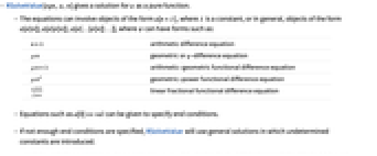
- The equations can involve objects of the form a[n+λ], where λ is a constant, or in general, objects of the form a[ψ[n]], a[ψ[ψ[n]]], a[ψ[…[ψ[n]]…]], where ψ can have forms such as:
-
n+λ arithmetic difference equation μ n geometric or  -difference equation
μ n+λ arithmetic-geometric functional difference equation μ nα geometric-power functional difference equation 
linear fractional functional difference equation - Equations such as a[0]==val can be given to specify end conditions.
- If not enough end conditions are specified, RSolveValue will use general solutions in which undetermined constants are introduced.
- The specification a∈Vectors[p] or a∈Matrices[{m,p}] can be used to indicate that the dependent variable a is a vector-valued or a matrix-valued variable, respectively. Alternatively, a can be specified as a VectorSymbol or MatrixSymbol. » »
- The constants introduced by RSolveValue are indexed by successive integers. The option GeneratedParameters specifies the function to apply to each index. The default is GeneratedParameters->C, which yields constants C[1], C[2], ….
- GeneratedParameters->(Module[{C},C]&) guarantees that the constants of integration are unique, even across different invocations of RSolveValue.
- For partial recurrence equations, RSolveValue generates arbitrary functions C[n][…].
- Solutions given by RSolveValue sometimes include sums that cannot be carried out explicitly by Sum. Dummy variables with local names are used in such sums.
- RSolveValue[eqn,a[Infinity],n] gives the limiting value of the solution a at Infinity.
- RSolveValue handles both ordinary difference equations and
 ‐difference equations.
 - RSolveValue handles difference‐algebraic equations, as well as ordinary difference equations.
- RSolveValue can solve linear recurrence equations of any order with constant coefficients. It can also solve many linear equations up to second order with nonconstant coefficients, as well as many nonlinear equations.
- RSolveValue[u[t]sys,resp,t] can be used for solving discrete-time models, where sys can be a TransferFunctionModel or a StateSpaceModel and the response function resp can be one of the following: »
-
"StateResponse" state response of sys to the input 
"OutputResponse" output response of sys to the input 
Examples
open all close allBasic Examples (4)
Scope (54)
Basic Uses (9)
Compute the general solution of a first-order difference equation:
Obtain a particular solution by adding an initial condition:
Plot the solution of a first-order difference equation:
Verify the solution of a difference equation by using a in the second argument:
Obtain the general solution of a higher-order difference equation:
Solve a system of difference equations:
Compute the value of the solution at a point:
Compute the limiting value of the solution at Infinity:
Solve a partial difference equation:
Use different names for the arbitrary constants in the general solution:
Linear Difference Equations (7)
First-order equation with variable coefficients:
A third-order constant coefficient equation:
Second-order inhomogeneous equation:
Second-order variable coefficient equation in terms of elementary functions:
In general, special functions are required to express solutions:
Higher-order inhomogeneous equation with constant coefficients:
Nonlinear Difference Equations (5)
Systems of Difference Equations (8)
Linear system with constant coefficients:
Variable coefficient linear system with a polynomial solution:
Linear constant coefficient difference-algebraic system:
Solve a linear system using vector variables:
Alternatively, define ![]() as a VectorSymbol:
as a VectorSymbol:
Solve a linear system using matrix variables:
Alternatively, define ![]() as a MatrixSymbol:
as a MatrixSymbol:
Solve an inhomogeneous linear system of ODEs with constant coefficients:
Partial Difference Equations (3)
Q–Difference Equations (6)
Functional Difference Equations (4)
Limits of Recursive Sequences (5)
Compute the limit of a linear recursive sequence:
Visualize the convergence of the sequence to its limiting value:
Compute the limit of a nonlinear recursive sequence:
Visualize the convergence of the sequence to its limiting value:
Compute the limit of a trigonometric recursive sequence:
Visualize the convergence of the sequence to its limiting value:
Compute the limit of a second-order recursive sequence:
Visualize the convergence of the sequence to its limiting value:
Compute the limit of the ratio of adjacent terms, f[n+1]/f[n], for the Fibonacci sequence, which satisfies the difference equation:
Solve the difference equation to find the ratio:
Compute the limit of the ratio using DiscreteLimit:
Visualize the convergence of the sequence to its limiting value:
Alternatively, compute the limit using DiscreteLimit in RSolveValue itself:
System Models (7)
Calculate the OutputResponse and StateResponse of a discrete-time StateSpaceModel for a sinusoidal input:
The output response of a transfer function model to a sinusoidal input:
The response of a state-space model from nonzero initial conditions:
The state response of a single-input system to a unit step input:
Plot the response for eight steps:
The state response for a generic discrete-time system:
The output response to a unit step sequence:
The output response of a discrete-time system to a time-dependent input:
Generalizations & Extensions (2)
Options (3)
Method (1)
Solve a linear ordinary difference equation:
Obtain a solution in terms of DifferenceRoot:
Assumptions (1)
Solve a second-order linear ordinary difference equation:
Use Assumptions to specify that the parameter λ is positive:
Applications (13)
This models the amount a[n] at year n when the interest r is paid on the principal p only:
Here the interest is paid on the current amount a[n], i.e. compound interest:
Here a[n] denotes the number of moves required in the Tower of Hanoi problem with n disks:
Here a[n] is the number of ways to tile an n×3 space with 2×1 tiles:
The number of comparisons for a binary search problem:
Number of arithmetic operations in the fast Fourier transform:
The nested radical ![]() satisfies a nonlinear difference equation:
satisfies a nonlinear difference equation:
Compute the exact value of the nested radical:
Visualize the convergence of the sequence to the exact value:
The integral ![]() satisfies the difference equation:
satisfies the difference equation:
The integral ![]() satisfies the difference equation:
satisfies the difference equation:
The difference equation for the series coefficients of ![]() :
:
The determinant of an n×n tridiagonal matrix with diagonals c, a, b satisfies:
This models the surface area s[n] in dimension n of a unit sphere:
The volume of the unit ball in dimension n:
Applying Newton's method to ![]() , or computing
, or computing ![]() :
:
Applying the Euler forward method to ![]() yields:
yields:
Solve the difference equation that describes the complexity of Karatsuba multiplication:
Compare with the complexity of schoolbook multiplication:
Efficiently compute the n![]() term of a linear recurrence for large n:
term of a linear recurrence for large n:
Properties & Relations (10)
RSolveValue returns an expression for the solution:
RSolve returns a rule for the solution:
Solutions satisfy their difference and boundary equations:
Difference equation corresponding to Sum:
Difference equation corresponding to Product:
RSolveValue finds a symbolic solution for this difference equation:
RecurrenceTable generates a procedural solution for the same problem:
FindLinearRecurrence finds the minimal linear recurrence for a list:
RSolveValue finds the sequence satisfying the recurrence:
LinearRecurrence generates the n![]() term for a linear recurrence:
term for a linear recurrence:
Obtain the same result using RSolveValue:
Use RecurrenceFilter to filter a signal:
Solve the corresponding difference equation using RSolveValue:
Forecast the next value for a time series based on ARProcess:
Obtain the same result using RSolveValue:
Use RFixedPoints to find the fixed points for a system of two recurrence equations:
Use RStabilityConditions to analyze the stability of the fixed point:
Solve the system using a fixed point as the initial condition:
Possible Issues (4)
Capital ![]() and capital
and capital ![]() cannot be used as independent variables:
cannot be used as independent variables:
Replacing them by lowercase ![]() or lowercase
or lowercase ![]() fixes the issue:
fixes the issue:
The solution to this difference equation is unique as a sequence:
As a function it is only unique up to a function of period 1:
RSolveValue returns only a single branch if the solution has multiple branches:
Use RSolve to get all of the solution branches:
Verify the solution when the equation involves subscripted variables:
Related Guides
History
Introduced in 2014 (10.0) | Updated in 2017 (11.2) ▪ 2022 (13.1) ▪ 2023 (13.3) ▪ 2024 (14.0) ▪ 2025 (14.2)
Text
Wolfram Research (2014), RSolveValue, Wolfram Language function, https://reference.wolfram.com/language/ref/RSolveValue.html (updated 2025).
CMS
Wolfram Language. 2014. "RSolveValue." Wolfram Language & System Documentation Center. Wolfram Research. Last Modified 2025. https://reference.wolfram.com/language/ref/RSolveValue.html.
APA
Wolfram Language. (2014). RSolveValue. Wolfram Language & System Documentation Center. Retrieved from https://reference.wolfram.com/language/ref/RSolveValue.html
BibTeX
@misc{reference.wolfram_2025_rsolvevalue, author="Wolfram Research", title="{RSolveValue}", year="2025", howpublished="\url{https://reference.wolfram.com/language/ref/RSolveValue.html}", note=[Accessed: 03-May-2026]}
BibLaTeX
@online{reference.wolfram_2025_rsolvevalue, organization={Wolfram Research}, title={RSolveValue}, year={2025}, url={https://reference.wolfram.com/language/ref/RSolveValue.html}, note=[Accessed: 03-May-2026]}