



ListVectorDensityPlot
ListVectorDensityPlot[varr]
ベクトル場とスカラー場の値{{vxij,vyij},rij}の配列 varr からベクトル密度プロットを生成する.
ListVectorDensityPlot[{{{x1,y1},{{vx1,vy1},r1}},…}]
指定の点{xi,yi}で与えられるベクトル場とスカラー場の値{{vxi,vyi},ri}からベクトル密度プロットを生成する.
ListVectorDensityPlot[{data1,data2,…}]
複数のベクトル場とスカラー場のデータをプロットする.
詳細とオプション
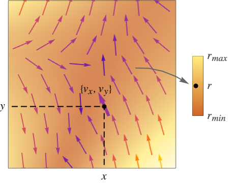
- ListVectorDensityPlotはスカラー場の背景濃度のプロットに重ね合されたベクトル場のベクトルプロットを生成する.
- ListVectorDensityPlotは,固定長に正規化された矢印を描くことでベクトル場を表示する.矢印は,デフォルトで,ベクトル場の強度
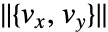 に従って彩色される.ベクトルはスカラー場 r の密度プロット上に描かれる.
- ベクトル場の強度
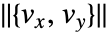 は,デフォルトで,スカラー場 r に使われる.
- プロットは集合
 を可視化する.
 は
 が定義されている領域である.
- ListVectorDensityPlotはデータをベクトル関数
 とスカラー関数
 に補間する.
- 規則的なデータについては,ベクトル場
 は値varr〚i,j,1〛を,スカラー場は値 varr〚i,j,2〛を
 で持つ.
- 不規則データについては,ベクトル場
 は値{vxi,vyi}を,スカラー場は値 riを
 で持つ.
- スカラー場の値が与えられていない場合,その値はベクトル場の法線であるとされる.
- ListVectorDensityPlot[varr]は連続する varr の行をページの上方向に,連続する列を横方向に並べる.
- ListVectorDensityPlotはデフォルトで,与えられたデータを補間し,構造格子位置でベクトル場のベクトルをプロットする.
- VectorPoints->Allの設定では,ListVectorDensityPlotは代りに与えられた特定のベクトル場のデータ点に関連するベクトルを示す.
- ListVectorDensityPlotにはGraphicsと同じオプションに次の追加・変更を加えたものが使える. [全オプションのリスト]
- MeshFunctions,RegionFunction,ColorFunction,VectorColorFunction中の関数に渡される引数は x, y, vx, vy, r である.
- デフォルト設定のMeshFunctions->{#5&}ではスカラー場 r にメッシュラインが描かれる.
- 次は,ScalingFunctionsの可能な設定である.
-
{sx,sy} x 軸と y 軸をスケールする - 次は,よく使われる組込みのスケーリング関数 s である.
-
"Log" 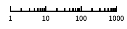
自動目盛ラベル付きの対数スケール "Log10" 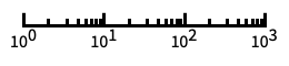
10のベキ乗に目盛が付いた,10を底とする対数スケール "SignedLog" 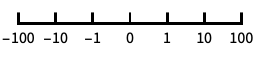
0と負の数を含む対数に似たスケール "Reverse" 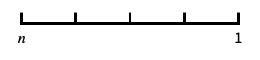
座標の向きを逆にする "Infinite" 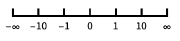
無限スケール
全オプションのリスト
例題
すべて開く すべて閉じる例 (2)
ノルムを指定されたベクトル集合から補間された背景としてベクトル場をプロットする:
ListVectorDensityPlot[Table[{y, -x}, {x, -3, 3, 0.2}, {y, -3, 3, 0.2}]]座標とベクトルを指定するデータからベクトル場をプロットする:
data = Table[{{x, y}, {y, x - x ^ 3}}, {x, -1.5, 1.5, 0.2}, {y, -2, 2, 0.2}];ListVectorDensityPlot[data]スコープ (20)
サンプリング (9)
ベクトルの規則的な集合の流線をプロットし,領域のデータ範囲を返す:
ListVectorDensityPlot[Table[{y, -x}, {x, -3, 3, 0.2}, {y, -3, 3, 0.2}], DataRange -> {{-3, 3}, {-3, 3}}]data = Table[{{x, y} = RandomReal[{-3, 3}, {2}], {y, -x}}, {200}];ListVectorDensityPlot[data]ListVectorDensityPlot[data, VectorPoints -> All]ListVectorDensityPlot[data, VectorPoints -> {4, 7}]data = Table[{{x, y}, {{y, x - x ^ 3}, Abs[x]}}, {x, -1.5, 1.5, 0.2}, {y, -2, 2, 0.2}];ListVectorDensityPlot[data]data = Table[{{x, y} = RandomReal[{-1.5, 1.5}, {2}], {{y, x - x ^ 3}, Abs[x]}}, {300}];ListVectorDensityPlot[data, VectorPoints -> All]2つのベクトル場を,最初のベクトル場のノルムに基づいた背景とともにプロットする:
data1 = Table[{{x, y} = RandomReal[{-3, 3}, {2}], {y, -x}}, {200}];
data2 = Table[{{x, y} = RandomReal[{-3, 3}, {2}], {y ^ 2, x - y}}, {150}];ListVectorDensityPlot[{data1, data2}, VectorPoints -> 10]ListVectorDensityPlot[Table[{y, -x}, {x, -3, 3, 0.2}, {y, -3, 3, 0.2}], DataRange -> {{-3, 3}, {-3, 3}}, VectorPoints -> RandomReal[{-3, 3}, {300, 2}]]data = Table[{y, -x}, {x, -2, 2, 0.2}, {y, -2, 2, 0.2}];Table[ListVectorDensityPlot[data, PlotLabel -> p, VectorPoints -> p], {p, {5, Coarse, Automatic, Fine}}]points = {{-1, -1}, {-1, 1}, {1, -1}, {1, 1}};
data = Table[{-1 - x ^ 2 + y, 1 + x - y ^ 2}, {x, -3, 3, 0.2}, {y, -3, 3, 0.2}];ListVectorDensityPlot[data, DataRange -> {{-3, 3}, {-3, 3}}, VectorPoints -> points, VectorSizes -> 2, Epilog -> {Red, PointSize[Medium], Point[points]}]ListVectorDensityPlot[Table[{{x, y} = RandomReal[{-3, 3}, {2}], {y, -x}}, {200}], RegionFunction -> Function[{x, y, vx, vy, n}, x y < 1]]プレゼンテーション (11)
ListVectorDensityPlot[Table[{y, -x}, {x, -3, 3, 0.2}, {y, -3, 3, 0.2}], VectorScaling -> Automatic]ListVectorDensityPlot[Table[{y, -x}, {x, -3, 3, 0.2}, {y, -3, 3, 0.2}], VectorColorFunction -> None]data = Table[{x, -y}, {x, -3, 3, 0.2}, {y, -3, 3, 0.2}];Table[ListVectorDensityPlot[data, VectorColorFunction -> Hue, PlotLabel -> s, VectorSizes -> s], {s, {Small, Medium, Large, 0.5}}]data = Table[{Sin[x], Cos[y]}, {x, -Pi, Pi, 0.2}, {y, -Pi, Pi, 0.2}];Table[ListVectorDensityPlot[data, PlotLabel -> s, VectorAspectRatio -> s], {s, {0.25, 0.5}}]場の強度によって背景とベクトルを彩色してベクトル場をプロットする:
VectorDensityPlot[{y, -x}, {x, -3, 3}, {y, -3, 3}, ColorFunction -> "Pastel", VectorColorFunction -> Hue]data1 = Table[{-1 - x ^ 2 + y, 1 + x - y ^ 2}, {x, -3, 3, 0.2}, {y, -3, 3, 0.2}];
data2 = Table[{-(1 + x - y ^ 2), -1 - x ^ 2 + y}, {x, -3, 3, 0.2}, {y, -3, 3, 0.2}];ListVectorDensityPlot[{data1, data2}, VectorPoints -> 8, VectorStyle -> {{Red, "Drop"}, {Blue, "Dart"}}, VectorColorFunction -> None]data = Table[{-1 - x ^ 2 + y, 1 + x - y ^ 2}, {x, -3, 3, 0.2}, {y, -3, 3, 0.2}];ListVectorDensityPlot[data, VectorPoints -> 8, VectorStyle -> Arrowheads[{{0.03, Automatic, Graphics[Circle[]]}}]]data = Table[{y, -x}, {x, -3, 3, 0.2}, {y, -3, 3, 0.2}];ListVectorDensityPlot[data, VectorMarkers -> "Drop"]ListVectorDensityPlot[data, VectorMarkers -> "Drop", VectorColorFunction -> None, VectorStyle -> Red]data = Table[{-1 - x ^ 2 + y, 1 + x - y ^ 2}, {x, -3, 3, 0.2}, {y, -3, 3, 0.2}];ListVectorDensityPlot[data, VectorStyle -> Red, VectorColorFunction -> None, PlotLegends -> Automatic]data = Table[{-1 - x ^ 2 + y, 1 + x - y ^ 2}, {x, -3, 3, 0.2}, {y, -3, 3, 0.2}];ListVectorDensityPlot[data, PlotTheme -> "Detailed"]コントラストがはっきりしたカラースキームとエッジフェイディングの矩形のテーマを使う:
data = Table[{-1 - x ^ 2 + y, 1 + x - y ^ 2}, {x, -3, 3, 0.2}, {y, -3, 3, 0.2}];ListVectorDensityPlot[data, PlotTheme -> "Marketing"]ListVectorDensityPlot[Flatten[Table[{{x, y}, {x, y - x}}, {x, -3, 3, 0.2}, {y, -3, 3, 0.2}], 1], ScalingFunctions -> {None, "Reverse"}]オプション (87)
Background (1)
BoundaryStyle (2)
data = Table[{Sin[x], Cos[y]}, {x, -3, 3, 0.2}, {y, -3, 3, 0.2}];ListVectorDensityPlot[data]data = Table[{Sin[x], Cos[y]}, {x, -3, 3, 0.2}, {y, -3, 3, 0.2}];ListVectorDensityPlot[data, BoundaryStyle -> Directive[Thick, Black]]ColorFunction (6)
Hueを使って場の強度に彩色する:
ListVectorDensityPlot[Table[{y, -x}, {x, -3, 3, 0.2}, {y, -3, 3, 0.2}], MaxRecursion -> 2, ColorFunction -> Hue] に基づいてHueを使って彩色する:
ListVectorDensityPlot[Table[{{y, -x}, Sin[x y]}, {x, -3, 3, 0.2}, {y, -3, 3, 0.2}], MaxRecursion -> 2, ColorFunction -> Hue]ColorDataから任意の名前付き色階調度を使う:
ListVectorDensityPlot[Table[{-1 - x ^ 2 + y, 1 + x - y ^ 2}, {x, -3, 3, 0.2}, {y, -3, 3, 0.2}], ColorFunction -> "Pastel"]定義済みの色階調度にColorDataを使う:
data = Table[{-1 - x ^ 2 + y, 1 + x - y ^ 2}, {x, -3, 3, 0.2}, {y, -3, 3, 0.2}];ListVectorDensityPlot[data, ColorFunction -> Function[{x, y, vx, vy, n}, ColorData["SolarColors"][x y]]]
data = Table[{-1 - x ^ 2 + y, 1 + x - y ^ 2}, {x, -3, 3, 0.2}, {y, -3, 3, 0.2}];ListVectorDensityPlot[data, ColorFunction -> Function[{x, y, vx, vy, n}, Blend[{Green, Red}, x]]]ColorFunctionScaling->Falseを使ってスケールされていない値を得る:
data = Table[{-1 - x ^ 2 + y, 1 + x - y ^ 2}, {x, -3, 3, 0.2}, {y, -3, 3, 0.2}];ListVectorDensityPlot[data, MaxRecursion -> 4, ColorFunctionScaling -> False, ColorFunction -> Function[{x, y, vx, vy, n}, ColorData[22][Round[n]]]]ColorFunctionScaling (4)
data = Table[{y Cos[x y], x Cos[x y]}, {x, -3, 3, 0.2}, {y, -3, 3, 0.2}];ListVectorDensityPlot[data, MaxRecursion -> 2, ColorFunction -> GrayLevel]ColorFunctionScaling->Falseを使ってスケールされていない値を得る:
data = Table[{y Cos[x y], x Cos[x y]}, {x, -3, 3, 0.2}, {y, -3, 3, 0.2}];ListVectorDensityPlot[data, MaxRecursion -> 4, ColorFunctionScaling -> False, ColorFunction -> Function[{x, y, vx, vy, n}, ColorData[22][Round[n]]]] 方向にスケールされていない座標を,
 方向にはスケールされた座標を使う:
data = Table[{y Cos[x y], x Cos[x y]}, {x, -3, 3, 0.2}, {y, -3, 3, 0.2}];ListVectorDensityPlot[data, ColorFunctionScaling -> {False, True}, ColorFunction -> Function[{x, y, vx, vy, n}, Hue[x, y, 1]]]data = Table[{y Cos[x y], x Cos[x y]}, {x, -3, 3, 0.2}, {y, -3, 3, 0.2}];ListVectorDensityPlot[data, MaxRecursion -> 3, ColorFunctionScaling -> {True, True, True, True, False}, ColorFunction -> Function[{x, y, vx, vy, n}, Hue[n, y, 1]]]DataRange (1)
EvaluationMonitor (1)
MaxRecursion (1)
Mesh (5)
ListVectorDensityPlot[Table[{-1 - x ^ 2 + y, 1 + x - y ^ 2}, {x, -3, 3, 0.2}, {y, -3, 3, 0.2}], Mesh -> None]Table[ListVectorDensityPlot[Table[{-1 - x ^ 2 + y, 1 + x - y ^ 2}, {x, -3, 3, 0.2}, {y, -3, 3, 0.2}], PlotLabel -> m, Mesh -> m], {m, {Full, Automatic}}]ListVectorDensityPlot[Table[{-1 - x ^ 2 + y, 1 + x - y ^ 2}, {x, -3, 3, 0.2}, {y, -3, 3, 0.2}], Mesh -> 5]ListVectorDensityPlot[Table[{-1 - x ^ 2 + y, 1 + x - y ^ 2}, {x, -3, 3, 0.2}, {y, -3, 3, 0.2}], Mesh -> {{2, 4, 5}}]data = Table[{-1 - x ^ 2 + y, 1 + x - y ^ 2}, {x, -3, 3, 0.2}, {y, -3, 3, 0.2}];ListVectorDensityPlot[data, Mesh -> {{{2, Thick}, {4, Yellow}, {5, {Thick, Red, Dashed}}}}]MeshFunctions (3)
data = Table[{-1 - x ^ 2 + y, 1 + x - y ^ 2}, {x, -3, 3, 0.2}, {y, -3, 3, 0.2}];ListVectorDensityPlot[data, Mesh -> 5, MeshFunctions -> Function[{x, y, vx, vy, n}, n]]
data = Table[{-1 - x ^ 2 + y, 1 + x - y ^ 2}, {x, -3, 3, 0.2}, {y, -3, 3, 0.2}];ListVectorDensityPlot[data, Mesh -> 5, MeshFunctions -> Function[{x, y, vx, vy, n}, x]]data = Table[{-1 - x ^ 2 + y, 1 + x - y ^ 2}, {x, -3, 3, 0.2}, {y, -3, 3, 0.2}];ListVectorDensityPlot[data, DataRange -> {{-3, 3}, {-3, 3}}, Mesh -> 5, MeshFunctions -> Function[{x, y, vx, vy, n}, Sqrt[x ^ 2 + y ^ 2]]]MeshShading (3)
Noneを使って範囲を削除する:
data = Table[{-1 - x ^ 2 + y, 1 + x - y ^ 2}, {x, -3, 3, 0.2}, {y, -3, 3, 0.2}];ListVectorDensityPlot[data, Mesh -> 10, MeshShading -> {Red, None}]data = Table[{-1 - x ^ 2 + y, 1 + x - y ^ 2}, {x, -3, 3, 0.2}, {y, -3, 3, 0.2}];ListVectorDensityPlot[data, Mesh -> 10, MeshShading -> {Red, Yellow, Green, None}]ColorDataからの指標付きの色を循環的に使う:
data = Table[{-1 - x ^ 2 + y, 1 + x - y ^ 2}, {x, -3, 3, 0.2}, {y, -3, 3, 0.2}];ListVectorDensityPlot[data, Mesh -> 10, MeshShading -> ColorData[51, "ColorList"]]MeshStyle (1)
PerformanceGoal (2)
ListVectorDensityPlot[Table[{-1 - x ^ 2 + y, 1 + x - y ^ 2}, {x, -3, 3, 0.2}, {y, -3, 3, 0.2}], PerformanceGoal -> "Quality"]ListVectorDensityPlot[Table[{-1 - x ^ 2 + y, 1 + x - y ^ 2}, {x, -3, 3, 0.2}, {y, -3, 3, 0.2}], PerformanceGoal -> "Speed"]PlotLegends (2)
ListVectorDensityPlot[Table[{-1 - x ^ 2 + y, 1 + x - y ^ 2}, {x, -2, 2, .2}, {y, -2, 2, .2}], PlotLegends -> Automatic]Placedを使って凡例をプロットの上に置く:
ListVectorDensityPlot[Table[{-1 - x ^ 2 + y, 1 + x - y ^ 2}, {x, -2, 2, .2}, {y, -2, 2, .2}], PlotLegends -> Placed[Automatic, Above]]PlotRange (7)
ListVectorDensityPlot[Table[{-1 - x ^ 2 + y, 1 + x - y ^ 2}, {x, -3, 3, 0.2}, {y, -3, 3, 0.2}], PlotRange -> Full]

ListVectorDensityPlot[Table[{-1 - x ^ 2 + y, 1 + x - y ^ 2}, {x, -3, 3, 0.2}, {y, -3, 3, 0.2}], DataRange -> {{-3, 3}, {-3, 3}}, PlotRange -> 2]
ListVectorDensityPlot[Table[{-1 - x ^ 2 + y, 1 + x - y ^ 2}, {x, -3, 3, 0.2}, {y, -3, 3, 0.2}], DataRange -> {{-3, 3}, {-3, 3}}, PlotRange -> {{-1, 2}, Automatic}]
ListVectorDensityPlot[Table[{-1 - x ^ 2 + y, 1 + x - y ^ 2}, {x, -3, 3, 0.2}, {y, -3, 3, 0.2}], DataRange -> {{-3, 3}, {-3, 3}}, PlotRange -> {{0, Full}, Automatic}]
ListVectorDensityPlot[Table[{-1 - x ^ 2 + y, 1 + x - y ^ 2}, {x, -3, 3, 0.2}, {y, -3, 3, 0.2}], DataRange -> {{-3, 3}, {-3, 3}}, PlotRange -> {Full, {0, 2}}]
ListVectorDensityPlot[Table[{-1 - x ^ 2 + y, 1 + x - y ^ 2}, {x, -3, 3, 0.2}, {y, -3, 3, 0.2}], DataRange -> {{-3, 3}, {-3, 3}}, PlotRange -> {Full, {Full, 5}}]

ListVectorDensityPlot[Table[{-1 - x ^ 2 + y, 1 + x - y ^ 2}, {x, -3, 3, 0.2}, {y, -3, 3, 0.2}], DataRange -> {{-3, 3}, {-3, 3}}, PlotRange -> {{-2, 1.5}, {-1, 2}}]PlotTheme (2)
単純な目盛,格子線,コントラストのはっきりしたカラースキームのテーマを使う:
ListVectorDensityPlot[Table[{-1 - x ^ 2 + y, 1 + x - y ^ 2}, {x, -3, 3, 0.2}, {y, -3, 3, 0.2}], DataRange -> {{-3, 3}, {-3, 3}}, PlotTheme -> "Business"]ListVectorDensityPlot[Table[{-1 - x ^ 2 + y, 1 + x - y ^ 2}, {x, -3, 3, 0.2}, {y, -3, 3, 0.2}], DataRange -> {{-3, 3}, {-3, 3}}, PlotTheme -> "Marketing"]RegionBoundaryStyle (4)
data = Table[{Cos[x], y}, {x, -3, 3, 0.2}, {y, -3, 3, 0.2}];ListVectorDensityPlot[data, DataRange -> {{-3, 3}, {-3, 3}}]data = Table[{Cos[x], y}, {x, -3, 3, 0.2}, {y, -3, 3, 0.2}];ListVectorDensityPlot[data, DataRange -> {{-3, 3}, {-3, 3}}, RegionFunction -> Function[{x, y, vx, vy, n}, x^2 + y^2 ≤ 9]]data = Table[{Cos[x], y}, {x, -3, 3, 0.2}, {y, -3, 3, 0.2}];ListVectorDensityPlot[data, DataRange -> {{-3, 3}, {-3, 3}}, RegionFunction -> Function[{x, y, vx, vy, n}, x^2 + y^2 ≤ 9], RegionBoundaryStyle -> Directive[Thick, Magenta]]data = Table[{Cos[x], y}, {x, -3, 3, 0.2}, {y, -3, 3, 0.2}];ListVectorDensityPlot[data, DataRange -> {{-3, 3}, {-3, 3}}, RegionBoundaryStyle -> Directive[Thick, Black]]RegionFunction (3)
data = Table[{-1 - x ^ 2 + y, 1 + x - y ^ 2}, {x, -3, 3, 0.2}, {y, -3, 3, 0.2}];ListVectorDensityPlot[data, DataRange -> {{-3, 3}, {-3, 3}}, RegionFunction -> Function[{x, y, vx, vy, n}, x y < 1]]場の強度が指定された閾値を超えている範囲のみでベクトルをプロットする:
data = Table[{-1 - x ^ 2 + y, 1 + x - y ^ 2}, {x, -3, 3, 0.2}, {y, -3, 3, 0.2}];ListVectorDensityPlot[data, DataRange -> {{-3, 3}, {-3, 3}}, RegionFunction -> Function[{x, y, vx, vy, n}, n > 6], MaxRecursion -> 1]data = Table[{-1 - x ^ 2 + y, 1 + x - y ^ 2}, {x, -3, 3, 0.2}, {y, -3, 3, 0.2}];ListVectorDensityPlot[data, DataRange -> {{-3, 3}, {-3, 3}}, RegionFunction -> Function[{x, y, vx, vy, n}, 4 < n < 9 || n < 2], MaxRecursion -> 2]ScalingFunctions (3)
ListVectorDensityPlot[Table[{y, x - y}, {x, -1, 1, 0.1}, {y, -1, 1, 0.1}]]ListVectorDensityPlot[Table[{y, x - y}, {x, -1, 1, 0.1}, {y, -1, 1, 0.1}], ScalingFunctions -> {None, "Log"}]ListVectorDensityPlot[Table[{y, x - y}, {x, -1, 1, 0.1}, {y, -1, 1, 0.1}], ScalingFunctions -> {None, "Reverse"}]VectorAspectRatio (1)
VectorAspectRatioを使って鏃の大きさを矢印の長さと相対的に指定する:
ListVectorDensityPlot[Table[{Sin[x], Cos[y]}, {x, -Pi, Pi, 0.2}, {y, -Pi, Pi, 0.2}], VectorAspectRatio -> 1 / 2]VectorColorFunction (4)
data = Table[{y, -x}, {x, -3, 3, 0.2}, {y, -3, 3, 0.2}];ListVectorDensityPlot[data, VectorColorFunction -> Hue]ColorDataから任意の名前付き色階調度を使う:
data = Table[{y, -x}, {x, -3, 3, 0.2}, {y, -3, 3, 0.2}];ListVectorDensityPlot[data, VectorColorFunction -> "Rainbow"]
data = Table[{y, -x}, {x, -3, 3, 0.2}, {y, -3, 3, 0.2}];ListVectorDensityPlot[data, VectorColorFunction -> Function[{x, y, vx, vy, n}, ColorData["ThermometerColors"][x]]]VectorColorFunctionScaling->Falseを使ってスケールされていない値を得る:
data = Table[{y, -x}, {x, -3, 3, 0.2}, {y, -3, 3, 0.2}];ListVectorDensityPlot[data, VectorColorFunction -> Function[{x, y, vx, vy, n}, ColorData[31][Round[n]]], VectorColorFunctionScaling -> False]VectorColorFunctionScaling (4)
ListVectorDensityPlot[Table[{y, -x}, {x, -3, 3, 0.2}, {y, -3, 3, 0.2}], VectorColorFunction -> Hue]VectorColorFunctionScaling->Falseを使ってスケールされていない値を得る:
data = Table[{y, -x}, {x, -3, 3, 0.2}, {y, -3, 3, 0.2}];ListVectorDensityPlot[data, VectorColorFunction -> Function[{x, y, vx, vy, n}, ColorData[31][Round[n]]], VectorColorFunctionScaling -> False] 方向にスケールされていない座標を,
 方向にはスケールされた座標を使う:
data = Table[{y, -x}, {x, 0, 1, 0.1}, {y, 0, 1, 0.1}];ListVectorDensityPlot[data, DataRange -> {{0, 2}, {0, 2}}, VectorColorFunction -> Function[{x, y, vx, vy, n}, Hue[x, y, 1]], VectorColorFunctionScaling -> {False, True}]data = Table[{y, -x}, {x, 0, 1, 0.1}, {y, 0, 1, 0.1}];ListVectorDensityPlot[data, DataRange -> {{0, 2}, {0, 2}}, VectorColorFunction -> Function[{x, y, vx, vy, n}, Hue[n, y, 1]], VectorColorFunctionScaling -> {True, True, True, True, False}]VectorMarkers (10)
data = Table[{y, -x}, {x, -3, 3, 0.2}, {y, -3, 3, 0.2}];ListVectorDensityPlot[data]data = Table[{y, -x}, {x, -3, 3, 0.2}, {y, -3, 3, 0.2}];ListVectorDensityPlot[data, VectorMarkers -> "Drop"]data1 = Table[{{x, y}, {y, -x}}, {x, -5, 5}, {y, -5, 5}];
data2 = Table[{{x, y}, {x, y}}, {x, -5, 5}, {y, -5, 5}];ListVectorDensityPlot[{data1, data2}, VectorMarkers -> {"Drop", "Dart"}]data = Table[{{x, y}, {y, -x}}, {x, -5, 5}, {y, -5, 5}];pts = Tuples[Range[-5, 5], 2];ListVectorDensityPlot[data, VectorMarkers -> "Arrow", VectorPoints -> pts, Epilog -> {Red, Point[pts]}]ListVectorDensityPlot[data, VectorMarkers -> Placed["Arrow", "Start"], VectorPoints -> pts, Epilog -> {Red, Point[pts]}]ListVectorDensityPlot[data, VectorMarkers -> Placed["Arrow", "End"], VectorPoints -> pts, Epilog -> {Red, Point[pts]}]ListVectorDensityPlot[Table[{-1 - x ^ 2 + y, 1 + x - y ^ 2}, {x, -3, 3, 0.2}, {y, -3, 3, 0.2}], VectorStyle -> "Segment"]data = Table[{-1 - x ^ 2 + y, 1 + x - y ^ 2}, {x, -3, 3, 0.2}, {y, -3, 3, 0.2}];Table[ListVectorDensityPlot[data, VectorPoints -> 8, PlotLabel -> s, VectorStyle -> s], {s, {"Arrow", "DotArrow", "ArrowArrow"}}]data = Table[{-1 - x ^ 2 + y, 1 + x - y ^ 2}, {x, -3, 3, 0.2}, {y, -3, 3, 0.2}];Table[ListVectorDensityPlot[data, VectorPoints -> 10, PlotLabel -> s, VectorStyle -> s], {s, {"Circle", "Disk", "CircleArrow"}}]data = Table[{-1 - x ^ 2 + y, 1 + x - y ^ 2}, {x, -3, 3, 0.2}, {y, -3, 3, 0.2}];Table[ListVectorDensityPlot[data, VectorPoints -> 8, PlotLabel -> s, VectorStyle -> s], {s, {"Dart", "PinDart", "DoubleDart"}}]data = Table[{-1 - x ^ 2 + y, 1 + x - y ^ 2}, {x, -3, 3, 0.2}, {y, -3, 3, 0.2}];Table[ListVectorDensityPlot[data, VectorPoints -> 8, PlotLabel -> s, VectorStyle -> s], {s, {"BarDot", "Dot", "DotArrow", "DotDot"}}]data = Table[{-1 - x ^ 2 + y, 1 + x - y ^ 2}, {x, -3, 3, 0.2}, {y, -3, 3, 0.2}];Table[ListVectorDensityPlot[data, VectorPoints -> 8, PlotLabel -> s, VectorStyle -> s], {s, {"Drop", "Pointer", "BackwardPointer", "Toothpick"}}]VectorPoints (8)
ListVectorDensityPlot[Table[{y, -x}, {x, -1, 1, 0.2}, {y, -1, 1, 0.2}], VectorPoints -> Automatic]ListVectorDensityPlot[Table[{y, -x}, {x, -1, 1, 0.2}, {y, -1, 1, 0.2}], VectorPoints -> All]data = Table[{y, -x}, {x, -3, 3, 0.2}, {y, -3, 3, 0.2}];Table[ListVectorDensityPlot[data, PlotLabel -> k, VectorPoints -> k], {k, {Fine, Coarse}}] と
 について同数の矢印を持つ場のベクトルの六角造格子を作成する:
ListVectorDensityPlot[Table[{y, -x}, {x, -3, 3, 0.2}, {y, -3, 3, 0.2}], VectorPoints -> 5] と
 について異なる数の矢印を持つ場のベクトルの六角格子を作成する:
ListVectorDensityPlot[Table[{y, -x}, {x, -3, 3, 0.2}, {y, -3, 3, 0.2}], VectorPoints -> {4, 7}]data = Table[{-1 - x ^ 2 + y, 1 + x - y ^ 2}, {x, -3, 3, 0.2}, {y, -3, 3, 0.2}];ListVectorDensityPlot[data, DataRange -> {{-3, 3}, {-3, 3}}, VectorPoints -> RandomReal[{-3, 3}, {300, 2}]]data = Table[{y ^ 2, x ^ 2 - y ^ 2}, {x, -3, 3, 0.2}, {y, -3, 3, 0.2}];Table[ListVectorDensityPlot[data, PlotLabel -> n, VectorPoints -> n, MaxRecursion -> 3], {n, 5, 20, 5}]data = Table[{-1 - x ^ 2 + y, 1 + x - y ^ 2}, {x, -3, 3, 0.2}, {y, -3, 3, 0.2}];
points = {{-1, -1}, {-1, 1}, {1, -1}, {1, 1}};ListVectorDensityPlot[data, DataRange -> {{-2, 2}, {-2, 2}}, VectorPoints -> points, VectorSizes -> 2, Epilog -> {Red, PointSize[Medium], Point[points]}]VectorScaling (2)
ListVectorDensityPlot[Table[{y, -x}, {x, -3, 3, 0.2}, {y, -3, 3, 0.2}], DataRange -> {{-3, 3}, {-3, 3}}]ListVectorDensityPlot[Table[{y, -x}, {x, -3, 3, 0.2}, {y, -3, 3, 0.2}], DataRange -> {{-3, 3}, {-3, 3}}, VectorScaling -> Automatic]VectorSizes (2)
data = Table[{Sin[x], Cos[y]}, {x, -Pi, Pi, 0.2}, {y, -Pi, Pi, 0.2}];Table[ListVectorDensityPlot[data, VectorPoints -> 10, PlotLabel -> s, VectorSizes -> s], {s, {0.5, 1}}]data = Table[{y, -x}, {x, -3, 3, 0.2}, {y, -3, 3, 0.2}];Table[ListVectorDensityPlot[data, VectorSizes -> s, PlotLabel -> s], {s, {Tiny, Small, Medium, Large}}]VectorStyle (5)
ListVectorDensityPlot[Table[{-1 - x ^ 2 + y, 1 + x - y ^ 2}, {x, -3, 3, 0.2}, {y, -3, 3, 0.2}], VectorColorFunction -> None, VectorStyle -> Blue]data1 = Table[{-1 - x ^ 2 + y, 1 + x - y ^ 2}, {x, -3, 3, 0.2}, {y, -3, 3, 0.2}];
data2 = Table[{-(1 + x - y ^ 2), -1 - x ^ 2 + y}, {x, -3, 3, 0.2}, {y, -3, 3, 0.2}];ListVectorDensityPlot[{data1, data2}, VectorColorFunction -> None, VectorStyle -> {Red, Blue}]Arrowheadsを使って鏃の明示的なスタイルを指定する:
data = Table[{x, y}, {x, -1, 1, 0.2}, {y, -1, 1, 0.2}];ListVectorDensityPlot[data, VectorStyle -> Arrowheads[{{0.02, Automatic, Graphics[Circle[]]}}]]data = Table[{x, y}, {x, -1, 1, 0.2}, {y, -1, 1, 0.2}];ListVectorDensityPlot[data, VectorPoints -> 9, VectorStyle -> Arrowheads[{{0.03, Automatic, Graphics[Rectangle[{-0.5, -0.5}, {0.5, 0.5}]]}, {0.03, Automatic, Graphics[Circle[]]}}]]Arrowheadsのないグラフィックスプリミティブはベクトルスケールに基づいてスケールされる:
data = Table[{x, y}, {x, -1, 1, 0.2}, {y, -1, 1, 0.2}];ListVectorDensityPlot[data, VectorStyle -> Graphics[Circle[]]]アプリケーション (2)
f = {Sin[x] ^ 3, -Cos[y] ^ 2};
df = Div[f, {x, y}];
data = Table[{f, df}, {x, -3, 3}, {y, -3, 3}];ListVectorDensityPlot[data]{dx, dy} = Table[ImageAdjust@GaussianFilter[[image], {6, 2}, δ], {δ, {{1, 0}, {0, 1}}}]data = Reverse /@ Transpose[2ImageData /@ {dx, dy} - 1, {3, 2, 1}];ListVectorDensityPlot[data, VectorPoints -> 30, ColorFunction -> "Rainbow", VectorScaling -> Automatic, VectorAspectRatio -> 1 / 2]特性と関係 (10)
VectorDensityPlotを使って関数をスカラー場の密度プロットともにプロットする:
VectorDensityPlot[{-1 - x ^ 2 + y, 1 + x - y ^ 2}, {x, -3, 3}, {y, -3, 3}]StreamDensityPlotを使ってベクトルの代りに流線をプロットする:
StreamDensityPlot[{-1 - x ^ 2 + y, 1 + x - y ^ 2}, {x, -3, 3}, {y, -3, 3}]密度プロットなしのデータのプロットにListVectorPlotを使う:
data = Table[{{x, y} = RandomReal[{-1.5, 1.5}, {2}], {{-1 - x ^ 2 + y, 1 + x - y ^ 2}, Abs[x + y]}}, {300}];ListVectorPlot[data]ListStreamPlotを使ってベクトルの代りに流線をプロットする:
ListStreamPlot[data]ListStreamDensityPlotを使って,ベクトルの代りに流線でプロットする:
ListStreamDensityPlot[Table[{-1 - x ^ 2 + y, 1 + x - y ^ 2}, {x, -3, 3, 0.2}, {y, -3, 3, 0.2}]]VectorPlotを使って密度プロットなしで関数をプロットする:
VectorPlot[{-1 - x ^ 2 + y, 1 + x - y ^ 2}, {x, -3, 3}, {y, -3, 3}]ListVectorDisplacementPlotを使って変位ベクトル場に関連付けられた領域の変形を可視化する:
data2D = Table[{{x, y} = RandomReal[{-1, 1}, {2}], {y, x - x^3}}, {300}];data3D = Table[{{x, y, z} = RandomReal[{0, 1}, {3}], {y, x, -z}}, {300}];ListVectorDisplacementPlot[data2D, Disk[], VectorPoints -> Automatic]ListVectorDisplacementPlot3Dを使って変形を3Dで可視化する:
ListVectorDisplacementPlot3D[data3D, Cuboid[], VectorPoints -> "Boundary"]スカラー場はListDensityPlotを使ってそれ自身でプロットすることができる:
f = {-1 - x ^ 2 + y, 1 + x - y ^ 2};
s = Exp[Norm[f] / 10];data = Table[{f, s}, {x, -3, 3, 0.2}, {y, -3, 3, 0.2}];
scalarData = Table[s, {x, -3, 3, 0.2}, {y, -3, 3, 0.2}];{ListDensityPlot[scalarData, ColorFunction -> "Pastel"],
ListVectorDensityPlot[data, ColorFunction -> "Pastel"]}ListLineIntegralConvolutionPlotを使ってベクトル場データの線形積分たたみ込みをプロットする:
data = Table[{-1 - x ^ 2 + y, 1 + x - y ^ 2}, {x, -3, 3, .2}, {y, -3, 3, .2}];ListLineIntegralConvolutionPlot[data]ListVectorPlot3DとListStreamPlot3Dを使って3Dベクトル場のデータを可視化する:
data = Table[{z, -x, y}, {x, -1, 1, .1}, {y, -1, 1, .1}, {z, -1, 1, .1}];{ListVectorPlot3D[data], ListStreamPlot3D[data]}ListSliceVectorPlot3Dを使って曲面上にベクトルをプロットする:
ListSliceVectorPlot3D[Table[{y, -x, z}, {z, -1, 1, .1}, {y, -1, 1, .1}, {x, -1, 1, .1}], Sphere[], DataRange -> {{-1, 1}, {-1, 1}, {-1, 1}}]GeoVectorPlotを使って地図上にベクトルをプロットする:
GeoVectorPlot[GeoVector[GeoPosition[{{-54.79801473961214, -111.85053058521567},
    {-65.56940402358214, 162.89657500795147}, {-81.67990688759895, -93.36222177594851},
    {7.785750774919734, 95.44840765141487}, {-6.86571958448036, -40.946398330539864},
    { ... 904, "AngularDegrees"]},
   {0.9366099079317551, Quantity[357.70482317743733, "AngularDegrees"]},
   {0.8256817194791912, Quantity[242.07227508889662, "AngularDegrees"]},
{0.2661401145642981, Quantity[152.90003252279325, "AngularDegrees"]}}]]GeoStreamPlotを使ってベクトルの代りに流線をプロットする:
GeoStreamPlot[GeoVector[GeoPosition[{{-54.79801473961214, -111.85053058521567},
    {-65.56940402358214, 162.89657500795147}, {-81.67990688759895, -93.36222177594851},
    {7.785750774919734, 95.44840765141487}, {-6.86571958448036, -40.946398330539864},
    { ... 904, "AngularDegrees"]},
   {0.9366099079317551, Quantity[357.70482317743733, "AngularDegrees"]},
   {0.8256817194791912, Quantity[242.07227508889662, "AngularDegrees"]},
{0.2661401145642981, Quantity[152.90003252279325, "AngularDegrees"]}}]]テキスト
Wolfram Research (2008), ListVectorDensityPlot, Wolfram言語関数, https://reference.wolfram.com/language/ref/ListVectorDensityPlot.html (2022年に更新).
CMS
Wolfram Language. 2008. "ListVectorDensityPlot." Wolfram Language & System Documentation Center. Wolfram Research. Last Modified 2022. https://reference.wolfram.com/language/ref/ListVectorDensityPlot.html.
APA
Wolfram Language. (2008). ListVectorDensityPlot. Wolfram Language & System Documentation Center. Retrieved from https://reference.wolfram.com/language/ref/ListVectorDensityPlot.html