


ListStreamPlot3D
ListStreamPlot3D[varr]
plots streamlines for the vector field given as an array of vectors.
Details and Options
- ListStreamPlot3D is known as a 3D stream plot or streamline plot. Besides lines, streamlines can also be displayed as tubes (stream tubes) and ribbons (stream ribbons).
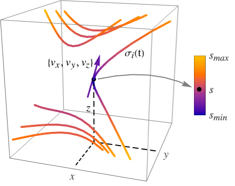
- ListStreamPlot3D plots streamlines
 defined by
  and
and  where
where  is an interpolated function of the vector data and
  is an initial stream point. The streamline
  is the curve passing through point
  , and whose tangents correspond to the vector field
  at each point.
 - The streamlines are colored by default according to the magnitude
 of the vector field
  and have an arrow in the direction of increasing value of
  .
. - The vector field
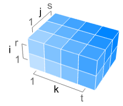
 has value varr〚i,j,k〛 at
  .
. - The varr represents vectors in a volume, where by default, the point {k,j,i} is taken to have the vector varr〚i,j,k〛 with 1≤i≤r, 1≤j≤s and 1≤k≤t for an array of dimension {r,s,t,3}.
- ListStreamPlot3D by default shows enough streamlines to achieve a roughly uniform density throughout the plot and shows no background scalar field.
- ListStreamPlot3D has the same options as Graphics3D, with the following additions and changes: [List of all options]
-
BoxRatios {1,1,1} ratio of height to width Method Automatic methods to use for the plot PerformanceGoal $PerformanceGoal aspects of performance to try to optimize PlotLegends None legends to include PlotRange {Full,Full,Full} range of x, y, z values to include PlotRangePadding Automatic how much to pad the range of values PlotTheme $PlotTheme overall theme for the plot RegionBoundaryStyle Automatic how to style plot region boundaries RegionFunction True& determine what region to include ScalingFunctions None how to scale individual coordinates StreamColorFunction Automatic how to color streamlines StreamColorFunctionScaling True whether to scale the argument to StreamColorFunction StreamMarkers Automatic shape to use for streams StreamPoints Automatic the number or placement of streamlines StreamScale None how to scale the sizes of streamlines StreamStyle Automatic how to draw streamlines - The arguments supplied to functions in RegionFunction and ColorFunction are x,y,z,vx,vy,vz,Norm[{vx,vy,vz}].
- Possible settings for StreamMarkers include:
-
"Arrow" lines with 2D arrowheads 
"Arrow3D" tubes with 3D arrowheads 
"Line" lines 
"Tube" tubes 
"Ribbon" flat ribbons 
"ArrowRibbon" ribbons with built-in arrowheads - With StreamScaleAutomatic and "arrow" stream markers, the streamlines are split into segments to make it easier to see the direction of the streamlines.
- Possible settings for StreamScale are:
-
Automatic automatically determine the streamline segments Full show the streamline as one piece Tiny,Small,Medium,Large named settings for how long the segments should be {len,npts,ratio} use explicit specification of streamline segmentation - The length len of streamline segments can be one of the following forms:
-
Automatic automatically determine the length None show the streamline as one piece Tiny,Small,Medium,Large use named segment lengths s use a length s that is a fraction of the graphic size - The number of points npts used to draw each segment can be Automatic or a specific number of points.
- The aspect ratio ratio specifies how wide the cross section of a streamline is relative to the streamline segment.
- Possible settings for ScalingFunctions are:
-
{sx,sy,sz} scale x, y and z axes - Common built-in scaling functions s include:
-
"Log" 
log scale with automatic tick labeling "Log10" 
base-10 log scale with powers of 10 for ticks "SignedLog" 
log-like scale that includes 0 and negative numbers "Reverse" 
reverse the coordinate direction "Infinite" 
infinite scale
List of all options
Examples
open all close allBasic Examples (4)
Plot the vector field interpolated from a specified set of vectors:
ListStreamPlot3D[Table[{z, -x, y}, {x, -1, 1, .1}, {y, -1, 1, .1}, {z, -1, 1, .1}]]Include a legend showing the field strength:
ListStreamPlot3D[Table[{x + y, y - z, x}, {x, -1, 1, .1}, {y, -1, 1, .1}, {z, -1, 1, .1}], PlotLegends -> Automatic]Use tubes to represent the streamlines:
ListStreamPlot3D[Table[{x, y + z, z}, {x, -1, 1, .1}, {y, -1, 1, .1}, {z, -1, 1, .1}], StreamMarkers -> "Tube"]Specify the range of the data:
ListStreamPlot3D[Table[{x, y, 1 + 2y}, {x, -1, 1, .1}, {y, -1, 1, .1}, {z, -1, 1, .1}], DataRange -> {{-1, 1}, {-1, 1}, {-1, 1}}]Scope (12)
Sampling (3)
Specify the density of seed points for the streamlines:
ListStreamPlot3D[Table[{2 , -Sin[π x], -x}, {x, -1, 1, 0.1}, {y, -1, 1, 0.1}, {z, -1, 1, 0.1}], StreamPoints -> Coarse]Specify specific seed points for the streamlines:
ListStreamPlot3D[Table[{2 , -Sin[π x], -x}, {x, -1, 1, 0.1}, {y, -1, 1, 0.1}, {z, -1, 1, 0.1}], StreamPoints -> RandomReal[{1, 20}, {30, 3}]]Plot streamlines over a specified region:
ListStreamPlot3D[Table[{2 , -Sin[π x], -x}, {x, -1, 1, 0.1}, {y, -1, 1, 0.1}, {z, -1, 1, 0.1}], RegionFunction -> Function[{x, y, z}, y ≥ x]]Presentation (9)
Streamlines are drawn as lines by default:
ListStreamPlot3D[Table[{x, y, 1 + 2y}, {x, -1, 1, 0.1}, {y, -1, 1, 0.1}, {z, -1, 1, 0.1}]]Use 3D tubes for the streamlines:
ListStreamPlot3D[Table[{x, y, 1 + 2y}, {x, -1, 1, 0.1}, {y, -1, 1, 0.1}, {z, -1, 1, 0.1}], StreamMarkers -> "Tube"]ListStreamPlot3D[Table[{x, y, 1 + 2y}, {x, -1, 1, 0.1}, {y, -1, 1, 0.1}, {z, -1, 1, 0.1}], StreamMarkers -> "Ribbon"]Use "arrow" versions of the stream markers to indicate the direction of flow along the streamlines:
ListStreamPlot3D[Table[{x, y, 1 + 2y}, {x, -1, 1, 0.1}, {y, -1, 1, 0.1}, {z, -1, 1, 0.1}], StreamMarkers -> "Arrow"]ListStreamPlot3D[Table[{x, y, 1 + 2y}, {x, -1, 1, 0.1}, {y, -1, 1, 0.1}, {z, -1, 1, 0.1}], StreamMarkers -> "Arrow3D"]Ribbons are turned into arrows by tapering the heads and notching the tails of the streamlines:
ListStreamPlot3D[Table[{x, y, 1 + 2y}, {x, -1, 1, 0.1}, {y, -1, 1, 0.1}, {z, -1, 1, 0.1}], StreamMarkers -> "ArrowRibbon"]Use a single color for the streamlines:
ListStreamPlot3D[Table[{x, y, 1 + 2y}, {x, -1, 1, 0.1}, {y, -1, 1, 0.1}, {z, -1, 1, 0.1}], StreamColorFunction -> None, StreamStyle -> RGBColor[0.09, 0.76, 0.65], StreamMarkers -> "Tube"]Use a named color gradient for the streamlines:
ListStreamPlot3D[Table[{x, y, 1 + 2y}, {x, -1, 1, 0.1}, {y, -1, 1, 0.1}, {z, -1, 1, 0.1}], StreamColorFunction -> "Rainbow"]Include a legend for the field magnitude:
ListStreamPlot3D[Table[{x, y, 1 + 2y}, {x, -1, 1, 0.1}, {y, -1, 1, 0.1}, {z, -1, 1, 0.1}], PlotLegends -> Automatic]Use StreamScale to split streamlines into multiple shorter line segments:
ListStreamPlot3D[Table[{x, y, 1 + 2y}, {x, -1, 1, 0.1}, {y, -1, 1, 0.1}, {z, -1, 1, 0.1}], StreamScale -> 0.1]ListStreamPlot3D[Table[{x, y, 1 + 2y}, {x, -1, 1, 0.1}, {y, -1, 1, 0.1}, {z, -1, 1, 0.1}], StreamScale -> 0.2]Increase the number of points in each segment and increase the marker aspect ratio:
ListStreamPlot3D[Table[{x, y, 1 + 2y}, {x, -1, 1, 0.1}, {y, -1, 1, 0.1}, {z, -1, 1, 0.1}], StreamMarkers -> "Arrow", StreamScale -> {Full, 20, 0.2}]ListStreamPlot3D[Table[{x, y, 1 + 2y}, {x, -1, 1, 0.1}, {y, -1, 1, 0.1}, {z, -1, 1, 0.1}], PlotTheme -> "Marketing"]Use a log scale in the z direction:
ListStreamPlot3D[Table[{x, y, 1 + 2y}, {x, -1, 1, 0.1}, {y, -1, 1, 0.1}, {z, -1, 1, 0.1}], ScalingFunctions -> {None, None, "Log"}]Options (75)
Axes (3)
By default, Axes are drawn:
ListStreamPlot3D[Table[{x, 2y, 3z}, {x, -2, 2, 0.1}, {y, -1, 1, 0.1}, {z, -1, 1, 0.1}]]Use AxesFalse to turn off axes:
ListStreamPlot3D[Table[{x, 2y, 3z}, {x, -2, 2, 0.1}, {y, -1, 1, 0.1}, {z, -1, 1, 0.1}], Axes -> False]Turn each axis on individually:
{ListStreamPlot3D[Table[{x, 2y, 3z}, {x, -2, 2, 0.1}, {y, -1, 1, 0.1}, {z, -1, 1, 0.1}], Axes -> {True, False, False}], ListStreamPlot3D[Table[{x, 2y, 3z}, {x, -2, 2, 0.1}, {y, -1, 1, 0.1}, {z, -1, 1, 0.1}], Axes -> {False, True, False}], ListStreamPlot3D[Table[{x, 2y, 3z}, {x, -2, 2, 0.1}, {y, -1, 1, 0.1}, {z, -1, 1, 0.1}], Axes -> {False, False, True}]}AxesLabel (4)
No axes labels are drawn by default:
ListStreamPlot3D[Table[{x, 2y, 3z}, {x, -2, 2, 0.1}, {y, -1, 1, 0.1}, {z, -1, 1, 0.1}]]ListStreamPlot3D[Table[{x, 2y, 3z}, {x, -2, 2, 0.1}, {y, -1, 1, 0.1}, {z, -1, 1, 0.1}], AxesLabel -> z]ListStreamPlot3D[Table[{x, 2y, 3z}, {x, -2, 2, 0.1}, {y, -1, 1, 0.1}, {z, -1, 1, 0.1}], AxesLabel -> {x, y, z}]ListStreamPlot3D[QuantityArray[Table[{x, 2y, 3z}, {x, -2, 2, 0.1}, {y, -1, 1, 0.1}, {z, -1, 1, 0.1}], "Meters"], AxesLabel -> Automatic]AxesOrigin (2)
The position of the axes is determined automatically:
ListStreamPlot3D[Table[{x, 2y, 3z}, {x, -2, 2, 0.1}, {y, -1, 1, 0.1}, {z, -1, 1, 0.1}]]Specify an explicit origin for the axes:
ListStreamPlot3D[Table[{x, 2y, 3z}, {x, -2, 2, 0.1}, {y, -1, 1, 0.1}, {z, -1, 1, 0.1}], AxesOrigin -> {1, 10, 10}]AxesStyle (4)
Change the style for the axes:
ListStreamPlot3D[Table[{x, 2y, 3z}, {x, -2, 2, 0.1}, {y, -1, 1, 0.1}, {z, -1, 1, 0.1}], AxesStyle -> StandardRed]Specify the style of each axis:
ListStreamPlot3D[Table[{x, 2y, 3z}, {x, -2, 2, 0.1}, {y, -1, 1, 0.1}, {z, -1, 1, 0.1}], AxesStyle -> {{Thick, StandardBrown}, {Thick, StandardBlue}, {Thick, StandardGreen}}]Use different styles for the ticks and the axes:
ListStreamPlot3D[Table[{x, 2y, 3z}, {x, -2, 2, 0.1}, {y, -1, 1, 0.1}, {z, -1, 1, 0.1}], AxesStyle -> StandardGreen, TicksStyle -> StandardGray]Use different styles for the labels and the axes:
ListStreamPlot3D[Table[{x, 2y, 3z}, {x, -2, 2, 0.1}, {y, -1, 1, 0.1}, {z, -1, 1, 0.1}], AxesStyle -> StandardGreen, LabelStyle -> StandardGray]BoxRatios (2)
By default, BoxRatios is set to Automatic:
ListStreamPlot3D[Table[{x, 2y, 3z}, {x, -2, 2, 0.1}, {y, -1, 1, 0.1}, {z, -1, 1, 0.1}]]Make the box twice as long in the x direction:
ListStreamPlot3D[Table[{x, 2y, 3z}, {x, -2, 2, 0.1}, {y, -1, 1, 0.1}, {z, -1, 1, 0.1}], BoxRatios -> {2, 1, 1}]DataRange (2)
By default, the data range is taken to be the index range of the data array:
ListStreamPlot3D[Table[{x - y, y - z, z - x}, {x, -2, 2, 0.1}, {y, -1, 1, 0.1}, {z, -1, 1, 0.1}]]Specify the data range for the domain:
ListStreamPlot3D[Table[{x - y, y - z, z - x}, {x, -2, 2, 0.1}, {y, -1, 1, 0.1}, {z, -1, 1, 0.1}], DataRange -> {{-2, 2}, {-1, 1}, {-1, 1}}]ImageSize (7)
Use named sizes such as Tiny, Small, Medium and Large:
{ListStreamPlot3D[Table[{x, 2y, 3z}, {x, -2, 2, 0.1}, {y, -1, 1, 0.1}, {z, -1, 1, 0.1}], ImageSize -> Tiny], ListStreamPlot3D[Table[{x, 2y, 3z}, {x, -2, 2, 0.1}, {y, -1, 1, 0.1}, {z, -1, 1, 0.1}], ImageSize -> Small]}Specify the width of the plot:
{ListStreamPlot3D[Table[{x, 2y, 3z}, {x, -2, 2, 0.1}, {y, -1, 1, 0.1}, {z, -1, 1, 0.1}], ImageSize -> 150], ListStreamPlot3D[Table[{x, 2y, 3z}, {x, -2, 2, 0.1}, {y, -1, 1, 0.1}, {z, -1, 1, 0.1}], AspectRatio -> 1.5, ImageSize -> 150]}Specify the height of the plot:
{ListStreamPlot3D[Table[{x, 2y, 3z}, {x, -2, 2, 0.1}, {y, -1, 1, 0.1}, {z, -1, 1, 0.1}], ImageSize -> {Automatic, 150}], ListStreamPlot3D[Table[{x, 2y, 3z}, {x, -2, 2, 0.1}, {y, -1, 1, 0.1}, {z, -1, 1, 0.1}], AspectRatio -> 2, ImageSize -> {Automatic, 150}]}Allow the width and height to be up to a certain size:
{ListStreamPlot3D[Table[{x, 2y, 3z}, {x, -2, 2, 0.1}, {y, -1, 1, 0.1}, {z, -1, 1, 0.1}], ImageSize -> UpTo[200]], ListStreamPlot3D[Table[{x, 2y, 3z}, {x, -2, 2, 0.1}, {y, -1, 1, 0.1}, {z, -1, 1, 0.1}], AspectRatio -> 2, ImageSize -> UpTo[200]]}Specify the width and height for a graphic, padding with space if necessary:
ListStreamPlot3D[Table[{x, 2y, 3z}, {x, -2, 2, 0.1}, {y, -1, 1, 0.1}, {z, -1, 1, 0.1}], ImageSize -> {200, 300}, Background -> StandardBlue]Setting AspectRatioFull will fill the available space:
ListStreamPlot3D[Table[{x, 2y, 3z}, {x, -2, 2, 0.1}, {y, -1, 1, 0.1}, {z, -1, 1, 0.1}], AspectRatio -> Full, ImageSize -> {200, 300}, Background -> StandardBlue]Use maximum sizes for the width and height:
{ListStreamPlot3D[Table[{x, 2y, 3z}, {x, -2, 2, 0.1}, {y, -1, 1, 0.1}, {z, -1, 1, 0.1}], ImageSize -> {UpTo[150], UpTo[100]}], ListStreamPlot3D[Table[{x, 2y, 3z}, {x, -2, 2, 0.1}, {y, -1, 1, 0.1}, {z, -1, 1, 0.1}], AspectRatio -> 2, ImageSize -> {UpTo[150], UpTo[100]}]}Use ImageSizeFull to fill the available space in an object:
Framed[Pane[ListStreamPlot3D[Table[{x, 2y, 3z}, {x, -2, 2, 0.1}, {y, -1, 1, 0.1}, {z, -1, 1, 0.1}], ImageSize -> Full, Background -> StandardBlue], {200, 100}]]Specify the image size as a fraction of the available space:
Framed[Pane[ListStreamPlot3D[Table[{x, 2y, 3z}, {x, -2, 2, 0.1}, {y, -1, 1, 0.1}, {z, -1, 1, 0.1}], AspectRatio -> Full, ImageSize -> {Scaled[0.5], Scaled[0.5]}, Background -> StandardBlue], {200, 200}]]PlotLegends (3)
No legends are included by default:
ListStreamPlot3D[Table[{1 - x, y - x, z - y}, {x, -1, 1, 0.1}, {y, -1, 1, 0.1}, {z, -1, 1, 0.1}]]Include a legend that indicates the vector field norm:
ListStreamPlot3D[Table[{1 - x, y - x, z - y}, {x, -1, 1, 0.1}, {y, -1, 1, 0.1}, {z, -1, 1, 0.1}], PlotLegends -> Automatic]Specify the location of the legend:
ListStreamPlot3D[Table[{1 - x, y - x, z - y}, {x, -1, 1, 0.1}, {y, -1, 1, 0.1}, {z, -1, 1, 0.1}], PlotLegends -> Placed[Automatic, Left]]PlotTheme (1)
RegionBoundaryStyle (4)
Show the region defined by a RegionFunction:
ListStreamPlot3D[Table[{1, -z, y}, {x, -2, 2, 0.5}, {y, -2, 2, 0.5}, {z, -2, 2, 0.5}], RegionFunction -> Function[{x, y, z, vx, vy, vz, n}, n < 2]]Use None to avoid showing the boundary:
ListStreamPlot3D[Table[{1, -z, y}, {x, -2, 2, 0.5}, {y, -2, 2, 0.5}, {z, -2, 2, 0.5}], RegionFunction -> Function[{x, y, z, vx, vy, vz, n}, n < 2], RegionBoundaryStyle -> None]Specify the color of the region boundary:
ListStreamPlot3D[Table[{1, -z, y}, {x, -2, 2, 0.5}, {y, -2, 2, 0.5}, {z, -2, 2, 0.5}], RegionFunction -> Function[{x, y, z, vx, vy, vz, n}, n < 2], RegionBoundaryStyle -> Yellow]The boundaries of full rectangular regions are not shown:
ListStreamPlot3D[Table[{1, -z, y}, {x, -2, 2, 0.5}, {y, -2, 2, 0.5}, {z, -2, 2, 0.5}]]RegionFunction (4)
Plot streamlines in a restricted region:
ListStreamPlot3D[Table[{y, -x, 3}, {x, -5, 5}, {y, -5, 5}, {z, -5, 5}], RegionFunction -> Function[{x, y, z, vx, vy, vz, n}, vx vy ≥ 0]]Plot streams only where the field magnitude exceeds a given threshold:
ListStreamPlot3D[Table[{y, -x, 3}, {x, -5, 5}, {y, -5, 5}, {z, -5, 5}], RegionFunction -> Function[{x, y, z, vx, vy, vz, n}, n ≥ 5]]Region functions depend, in general, on seven arguments:
ListStreamPlot3D[Table[{y, -x, 3}, {x, -5, 5}, {y, -5, 5}, {z, -5, 5}], RegionFunction -> Function[{x, y, z, vx, vy, vz, n}, 3n ≥ x + y]]Use RegionBoundaryStyleNone to avoid showing the boundary:
ListStreamPlot3D[Table[{y, -x, 3}, {x, -5, 5}, {y, -5, 5}, {z, -5, 5}], RegionFunction -> Function[{x, y, z, vx, vy, vz, n}, n ≥ 5], RegionBoundaryStyle -> None]ScalingFunctions (3)
By default, linear scales are used:
ListStreamPlot3D[Table[{x, y, 1 + 2y}, {x, -1, 1, 0.1}, {y, -1, 1, 0.1}, {z, -1, 1, 0.1}]]Use a log scale in the z direction:
ListStreamPlot3D[Table[{x, y, 1 + 2y}, {x, -1, 1, 0.1}, {y, -1, 1, 0.1}, {z, -1, 1, 0.1}], ScalingFunctions -> {None, None, "Log"}]Reverse the direction of the z direction:
ListStreamPlot3D[Table[{x, y, 1 + 2y}, {x, -1, 1, 0.1}, {y, -1, 1, 0.1}, {z, -1, 1, 0.1}], ScalingFunctions -> {None, None, "Reverse"}]StreamColorFunction (4)
Color the streams by their norm:
ListStreamPlot3D[Table[{3x, 2y, z}, {x, -1, 1, 0.1}, {y, -1, 1, 0.1}, {z, -1, 1, 0.1}], StreamColorFunction -> Hue]Use any named color gradient from ColorData:
ListStreamPlot3D[Table[{3x, 2y, z}, {x, -1, 1, 0.1}, {y, -1, 1, 0.1}, {z, -1, 1, 0.1}], StreamColorFunction -> "Rainbow"]Color the streamlines according to their x value:
ListStreamPlot3D[Table[{3x, 2y, z}, {x, -1, 1, 0.1}, {y, -1, 1, 0.1}, {z, -1, 1, 0.1}], StreamColorFunction -> Function[{x, y, z, vx, vy, vz, n}, Hue[x]]]Use StreamColorFunctionScalingFalse to get unscaled values:
ListStreamPlot3D[Table[{3x, 2y, z}, {x, -1, 1, 0.1}, {y, -1, 1, 0.1}, {z, -1, 1, 0.1}], StreamColorFunction -> "Rainbow", StreamColorFunctionScaling -> False]StreamColorFunctionScaling (2)
By default, scaled values are used:
ListStreamPlot3D[Table[{y, -x, E^z}, {x, -1, 1, 0.1}, {y, -1, 1, 0.1}, {z, -1, 1, 0.1}], StreamColorFunction -> "Pastel", PlotLegends -> Automatic]Use StreamColorFunctionScalingFalse to get unscaled values:
ListStreamPlot3D[Table[{y, -x, E^z}, {x, -1, 1, 0.1}, {y, -1, 1, 0.1}, {z, -1, 1, 0.1}], StreamColorFunction -> "Pastel", PlotLegends -> Automatic, StreamColorFunctionScaling -> False]StreamMarkers (5)
ListStreamPlot3D[Table[{E^x, E^y, -3}, {x, -1, 1, 0.1}, {y, -1, 1, 0.1}, {z, -1, 1, 0.1}]]Draw the streamlines as tubes:
ListStreamPlot3D[Table[{E^x, E^y, -3}, {x, -1, 1, 0.1}, {y, -1, 1, 0.1}, {z, -1, 1, 0.1}], StreamMarkers -> "Tube"]ListStreamPlot3D[Table[{E^x, E^y, -3}, {x, -1, 1, 0.1}, {y, -1, 1, 0.1}, {z, -1, 1, 0.1}], StreamMarkers -> "Ribbon"]"Arrow" stream markers automatically break the streamlines into shorter segments:
ListStreamPlot3D[Table[{E^x, E^y, -3}, {x, -1, 1, 0.1}, {y, -1, 1, 0.1}, {z, -1, 1, 0.1}], StreamMarkers -> "Arrow"]ListStreamPlot3D[Table[{E^x, E^y, -3}, {x, -1, 1, 0.1}, {y, -1, 1, 0.1}, {z, -1, 1, 0.1}], StreamMarkers -> "Arrow3D"]ListStreamPlot3D[Table[{E^x, E^y, -3}, {x, -1, 1, 0.1}, {y, -1, 1, 0.1}, {z, -1, 1, 0.1}], StreamMarkers -> "ArrowRibbon"]Make segmented markers continuous:
ListStreamPlot3D[Table[{E^x, E^y, -3}, {x, -1, 1, 0.1}, {y, -1, 1, 0.1}, {z, -1, 1, 0.1}], StreamMarkers -> "Arrow3D", StreamScale -> Full]Break continuous markers into segments:
ListStreamPlot3D[Table[{E^x, E^y, -3}, {x, -1, 1, 0.1}, {y, -1, 1, 0.1}, {z, -1, 1, 0.1}], StreamMarkers -> "Ribbon", StreamScale -> 0.1]StreamPoints (4)
Use automatically determined stream points to seed the curves:
ListStreamPlot3D[Table[{1, -E^-y, E^z}, {x, -2, 2, 0.1}, {y, -2, 2, 0.1}, {z, -2, 2, 0.1}]]Specify a maximum number of streamlines:
ListStreamPlot3D[Table[{1, -E^-y, E^z}, {x, -2, 2, 0.1}, {y, -2, 2, 0.1}, {z, -2, 2, 0.1}], StreamPoints -> 40]Give specific seed points for the streams:
ListStreamPlot3D[Table[{1, -E^-y, E^z}, {x, -2, 2, 0.1}, {y, -2, 2, 0.1}, {z, -2, 2, 0.1}], StreamPoints -> RandomReal[{1, 40}, {20, 3}]]Use coarsely spaced streamlines:
ListStreamPlot3D[Table[{1, -E^-y, E^z}, {x, -2, 2, 0.1}, {y, -2, 2, 0.1}, {z, -2, 2, 0.1}], StreamPoints -> Coarse]Use more finely spaced streamlines:
ListStreamPlot3D[Table[{1, -E^-y, E^z}, {x, -2, 2, 0.1}, {y, -2, 2, 0.1}, {z, -2, 2, 0.1}], StreamPoints -> Fine]StreamScale (9)
Segmented markers have default lengths, numbers of points and aspect ratios:
ListStreamPlot3D[Table[{y^2, -x^2, 2 - z}, {x, -1, 1, 0.1}, {y, -1, 1, 0.1}, {z, -1, 1, 0.1}], StreamMarkers -> "Arrow"]Modify the lengths of the segments:
ListStreamPlot3D[Table[{y^2, -x^2, 2 - z}, {x, -1, 1, 0.1}, {y, -1, 1, 0.1}, {z, -1, 1, 0.1}], StreamMarkers -> "Arrow", StreamScale -> 0.2]Specify the number of sample points in each segment:
ListStreamPlot3D[Table[{y^2, -x^2, 2 - z}, {x, -1, 1, 0.1}, {y, -1, 1, 0.1}, {z, -1, 1, 0.1}], StreamMarkers -> "Arrow", StreamScale -> {0.2, 2}]Modify the aspect ratios for the stream markers:
ListStreamPlot3D[Table[{y^2, -x^2, 2 - z}, {x, -1, 1, 0.1}, {y, -1, 1, 0.1}, {z, -1, 1, 0.1}], StreamMarkers -> "Arrow", StreamScale -> {0.2, 2, 0.2}]Make segmented markers continuous:
ListStreamPlot3D[Table[{y^2, -x^2, 2 - z}, {x, -1, 1, 0.1}, {y, -1, 1, 0.1}, {z, -1, 1, 0.1}], StreamMarkers -> "Arrow", StreamScale -> Full]Break continuous markers into segments:
ListStreamPlot3D[Table[{y^2, -x^2, 2 - z}, {x, -1, 1, 0.1}, {y, -1, 1, 0.1}, {z, -1, 1, 0.1}], StreamMarkers -> "Ribbon", StreamScale -> 0.2]The aspect ratio controls the thickness of ribbons and tubes:
ListStreamPlot3D[Table[{y^2, -x^2, 2 - z}, {x, -1, 1, 0.1}, {y, -1, 1, 0.1}, {z, -1, 1, 0.1}], StreamMarkers -> "ArrowRibbon", StreamScale -> {Automatic, Automatic, 0.05}]ListStreamPlot3D[Table[{y^2, -x^2, 2 - z}, {x, -1, 1, 0.1}, {y, -1, 1, 0.1}, {z, -1, 1, 0.1}], StreamMarkers -> "Ribbon", StreamScale -> {Automatic, Automatic, 0.05}]ListStreamPlot3D[Table[{y^2, -x^2, 2 - z}, {x, -1, 1, 0.1}, {y, -1, 1, 0.1}, {z, -1, 1, 0.1}], StreamMarkers -> "Tube", StreamScale -> {Automatic, Automatic, 0.05}]The aspect ratio controls the sizes of arrowheads:
ListStreamPlot3D[Table[{y^2, -x^2, 2 - z}, {x, -1, 1, 0.1}, {y, -1, 1, 0.1}, {z, -1, 1, 0.1}], StreamMarkers -> "Arrow", StreamScale -> {Automatic, Automatic, 0.2}]Use three points in each segment:
ListStreamPlot3D[Table[{y^2, -x^2, 2 - z}, {x, -1, 1, 0.1}, {y, -1, 1, 0.1}, {z, -1, 1, 0.1}], StreamMarkers -> "Arrow", StreamScale -> {0.5, 3}]StreamStyle (3)
Change the appearance of the streamlines:
ListStreamPlot3D[Table[{-y^2, x^2, 0.5}, {x, -1, 1, 0.1}, {y, -1, 1, 0.1}, {z, -1, 1, 0.1}], StreamStyle -> Thickness[0.02]]StreamColorFunction takes precedence over StreamStyle:
ListStreamPlot3D[Table[{-y^2, x^2, 0.5}, {x, -1, 1, 0.1}, {y, -1, 1, 0.1}, {z, -1, 1, 0.1}], StreamStyle -> Directive[Red, Dashing[{0.1, 0.02}]]]Use StreamColorFunctionNone to specify a streamline color with StreamStyle:
ListStreamPlot3D[Table[{-y^2, x^2, 0.5}, {x, -1, 1, 0.1}, {y, -1, 1, 0.1}, {z, -1, 1, 0.1}], StreamStyle -> Directive[StandardRed, Dashing[{0.1, 0.02}]], StreamColorFunction -> None]Ticks (6)
Ticks are placed automatically in each plot:
ListStreamPlot3D[Table[{x + y, y - z, x}, {z, -2, 2, 0.1}, {y, -2, 2, 0.1}, {x, -2, 2, 0.1}]]Use TicksNone to not draw any tick marks:
ListStreamPlot3D[Table[{x + y, y - z, x}, {z, -2, 2, 0.1}, {y, -2, 2, 0.1}, {x, -2, 2, 0.1}], Ticks -> None]Place tick marks at specific positions:
ListStreamPlot3D[Table[{x + y, y - z, x}, {z, -2, 2, 0.1}, {y, -2, 2, 0.1}, {x, -2, 2, 0.1}], Ticks -> {{5, 15, 25}, {5, 15, 25}, {5, 15, 25}}]Draw tick marks at the specified positions with the specified labels:
ListStreamPlot3D[Table[{x + y, y - z, x}, {z, -2, 2, 0.1}, {y, -2, 2, 0.1}, {x, -2, 2, 0.1}], Ticks -> {{{5, a}, {15, b}, {25, c}}, {{5, a}, {15, b}, {25, c}}, {{5, a}, {15, b}, {25, c}}}]Specify tick marks with scaled lengths:
ListStreamPlot3D[Table[{x + y, y - z, x}, {z, -2, 2, 0.1}, {y, -2, 2, 0.1}, {x, -2, 2, 0.1}], Ticks -> {{{5, a, .1}, {15, b, .1}, {25, c, .1}}, {{5, a, .05}, {15, b, .05}, {25, c, .05}}, {{5, a, .15}, {15, b, .15}, {25, c, .15}}}]Customize each tick with position, length, labeling and styling:
ListStreamPlot3D[Table[{x + y, y - z, x}, {z, -2, 2, 0.1}, {y, -2, 2, 0.1}, {x, -2, 2, 0.1}], Ticks -> {{{5, a, .1, Directive[Red]}, {15, b, .1, Directive[Red, Thick]}, {25, c, .1, Directive[Red, Dashed, Thick]}}, {{5, a, .1, Directive[Blue]}, {15, b, .1, Directive[Blue, Thick]}, {25, c, .1, Directive[Blue, Dashed, Thick]}}, {{5, a, .1, Directive[Darker@Green]}, {15, b, .1, Directive[Darker@Green, Thick]}, {25, c, .1, Directive[Darker@Green, Dashed, Thick]}}}]TicksStyle (3)
By default, the ticks and tick labels use the same styles as the axis:
ListStreamPlot3D[Table[{x + y, y - z, x}, {z, -2, 2, 0.1}, {y, -2, 2, 0.1}, {x, -2, 2, 0.1}], AxesStyle -> Directive[Thick, StandardRed]]Specify overall ticks style, including the tick labels:
ListStreamPlot3D[Table[{x + y, y - z, x}, {z, -2, 2, 0.1}, {y, -2, 2, 0.1}, {x, -2, 2, 0.1}], TicksStyle -> Directive[Bold, StandardRed]]Specify tick style for each of the axes:
ListStreamPlot3D[Table[{x + y, y - z, x}, {z, -2, 2, 0.1}, {y, -2, 2, 0.1}, {x, -2, 2, 0.1}], TicksStyle -> {Directive[StandardGray, Bold], Directive[Bold, StandardRed], Directive[Bold, StandardBlue]}]Applications (2)
Numerically compute the electric field at a sampling of points under the influence of two thin wires of finite length with equal constant charge densities and opposite signs:
data = Quiet@Table[If[Abs[x] == 1 && z == 0 && -2 ≤ y ≤ 2, {0, 0, 0}, NIntegrate[({x + 1, y - Y, z}/Norm[{x + 1, y - Y, z}]^3) - ({x - 1, y - Y, z}/Norm[{x - 1, y - Y, z}]^3), {Y, -2, 2}]], {x, -5, 5}, {y, -5, 5}, {z, -5, 5}];Visualize the electric field along with the positively charged (black) and the negatively charged (red) wires:
Show[ListStreamPlot3D[data, StreamMarkers -> "Arrow", DataRange -> {{-5, 5}, {-5, 5}, {-5, 5}}, StreamColorFunction -> None, StreamStyle -> StandardBlue], Graphics3D[{Thickness[0.01], Line[{{-1, -2, 0}, {-1, 2, 0}}], StandardRed, Line[{{1, -2, 0}, {1, 2, 0}}]}]]Visualize time-independent heat flow in a unit cube. Consider the steady-state heat equation ![]() for the temperature
for the temperature ![]() on the unit cube with
on the unit cube with ![]() on the
on the ![]() face, insulated on the
face, insulated on the ![]() ,
, ![]() ,
, ![]() and
and ![]() faces,
faces, ![]() inside a centered disk of radius 0.3 on the
inside a centered disk of radius 0.3 on the ![]() face and
face and ![]() outside the disk as shown in the following:
outside the disk as shown in the following:
cube = [image];Use finite differences to discretize the heat equation ![]() :
:
n = 20; (* number of steps *)
Δ = (1.0/n + 1); (* step size *)
vars = Flatten[Table[u[i, j, k], {i, 1, n}, {j, 0, n + 1}, {k, 0, n + 1}]];
eqns = Flatten[Table[
	u[i + 1, j, k] - 2u[i, j, k] + u[i - 1, j, k] + (* x direction *)
	u[i, j + 1, k] - 2u[i, j, k] + u[i, j - 1, k] + (* y direction *)
	u[i, j, k + 1] - 2u[i, j, k] + u[i, j, k - 1](* z direction *)
	 == 0, {i, 1, n}, {j, 0, n + 1}, {k, 0, n + 1}]];
Specify boundary conditions for ![]() on the
on the ![]() and
and ![]() faces:
faces:
u[0, _, _] := 1.0;
u[n + 1, j_, k_] := If[(j Δ - 0.5)^2 + (k Δ - 0.5)^2 ≤ 0.3^2, 2, 0];
Specify the insulated boundary conditions for ![]() on the other faces:
on the other faces:
u[i_, -1, k_] := u[i, 1, k];(* y=0 *)
u[i_, n + 2, k_] := u[i, n, k]; (* y=1 *)
u[i_, j_, -1] := u[i, j, 1]; (* z=0 *)
u[i_, j_, n + 2] := u[i, j, n];(* z=1 *)
Solve the system of equations:
sol = Solve[eqns, vars][[1]];
temperatures = Table[u[i, j, k], {k, 0, n + 1}, {j, 0, n + 1}, {i, 0, n + 1}] /. sol;
Use finite differences to approximate the heat flux:
heatflux = Table[-{(u[i + 1, j, k] - u[i - 1, j, k]/2Δ), (u[i, j + 1, k] - u[i, j - 1, k]/2Δ), (u[i, j, k + 1] - u[i, j, k - 1]/2Δ)} /. sol, {i, 1, n}, {j, 1, n}, {k, 1, n}];Generate seed points for the streamlines on the ![]() face:
face:
sp1 = Flatten[Table[{0, y, z}, {y, 0.1, 0.9, 0.2}, {z, 0.1, 0.9, 0.2}], 1];Generate seed points for the streamlines in the red disk on the ![]() face:
face:
sp2 = Flatten[Table[{1, 0.5 + r Cos[t], 0.5 + r Sin[t]}, {r, 0, 0.2, 0.1}, {t, 0, 2π - (π/5), (π/5)}], 1];Visualize the heat flow. The boundary temperatures are specified in the legend, and the blank faces of the cube are insulated:
Show[ListStreamPlot3D[heatflux, DataRange -> {{0, 1}, {0, 1}, {0, 1}}, StreamPoints -> Join[sp1, sp2], StreamMarkers -> "Arrow3D", StreamScale -> Full, StreamColorFunction -> None, StreamStyle -> RGBColor[0.8675693999999999, 0.4915453999999999, 0.21120899999999998]], cube, Lighting -> "Neutral"]Properties & Relations (10)
Use StreamPlot3D and VectorPlot3D to visualize functions:
{StreamPlot3D[{z, -x, y}, {x, -3, 3}, {y, -3, 3}, {z, -3, 3}], VectorPlot3D[{z, -x, y}, {x, -3, 3}, {y, -3, 3}, {z, -3, 3}]}Use StreamPlot and VectorPlot to visualize functions in 2D:
{StreamPlot[{y - x, y}, {x, -3, 3}, {y, -3, 3}], VectorPlot[{y - x, y}, {x, -3, 3}, {y, -3, 3}]}Plot vectors along surfaces with ListSliceVectorPlot3D:
data = Table[{-1 - x ^ 2 + y, 1 + x - y ^ 2, z}, {x, -3, 3}, {y, -3, 3}, {z, -3, 3}];ListSliceVectorPlot3D[data]Use ListVectorPlot3D to plot a 3D field as discrete vectors:
data = Table[{-1 - x ^ 2 + y, 1 + x - y ^ 2, z}, {x, -3, 3}, {y, -3, 3}, {z, -3, 3}];ListVectorPlot3D[data]Use ListVectorPlot for plotting 2D vectors:
data = Table[{-1 - x ^ 2 + y, 1 + x - y ^ 2}, {x, -3, 3}, {y, -3, 3}];ListVectorPlot[data]Use ListStreamPlot to plot with streamlines instead of vectors:
data = Table[{-1 - x ^ 2 + y, 1 + x - y ^ 2}, {x, -3, 3}, {y, -3, 3}];ListStreamPlot[data]Use ListVectorDensityPlot or ListStreamDensityPlot to add a density plot of a scalar field:
data = Table[{{-1 - x ^ 2 + y, 1 + x - y ^ 2}, Abs[x] + Abs[y]}, {x, -3, 3}, {y, -3, 3}];{ListVectorDensityPlot[data], ListStreamDensityPlot[data]}Use ListVectorDisplacementPlot to visualize the deformation of a region associated with a displacement vector field:
data2D = Table[{{x, y} = RandomReal[{-1, 1}, {2}], {y, x - x^3}}, {300}];data3D = Table[{{x, y, z} = RandomReal[{0, 1}, {3}], {y, x, -z}}, {300}];ListVectorDisplacementPlot[data2D, Disk[], VectorPoints -> Automatic]Use ListVectorDisplacementPlot3D to visualize a deformation in 3D:
ListVectorDisplacementPlot3D[data3D, Cuboid[], VectorPoints -> "Boundary"]Use ListLineIntegralConvolutionPlot to plot the line integral convolution of a vector field:
data = Table[{-1 - x ^ 2 + y, 1 + x - y ^ 2}, {x, -3, 3}, {y, -3, 3}];ListLineIntegralConvolutionPlot[data]Use GeoVectorPlot to plot vectors on a map:
GeoVectorPlot[GeoVector[GeoPosition[{{-54.79801473961214, -111.85053058521567},
    {-65.56940402358214, 162.89657500795147}, {-81.67990688759895, -93.36222177594851},
    {7.785750774919734, 95.44840765141487}, {-6.86571958448036, -40.946398330539864},
    { ... 904, "AngularDegrees"]},
   {0.9366099079317551, Quantity[357.70482317743733, "AngularDegrees"]},
   {0.8256817194791912, Quantity[242.07227508889662, "AngularDegrees"]},
   {0.2661401145642981, Quantity[152.90003252279325, "AngularDegrees"]}}]]
Use GeoStreamPlot to plot streamlines instead of vectors:
GeoStreamPlot[GeoVector[GeoPosition[{{-54.79801473961214, -111.85053058521567},
    {-65.56940402358214, 162.89657500795147}, {-81.67990688759895, -93.36222177594851},
    {7.785750774919734, 95.44840765141487}, {-6.86571958448036, -40.946398330539864},
    { ... 904, "AngularDegrees"]},
   {0.9366099079317551, Quantity[357.70482317743733, "AngularDegrees"]},
   {0.8256817194791912, Quantity[242.07227508889662, "AngularDegrees"]},
   {0.2661401145642981, Quantity[152.90003252279325, "AngularDegrees"]}}]]
Possible Issues (2)
Tube StreamMarkers can be distorted by the BoxRatios:
data = Table[{2, -10 z - x y, 10 y - x z}, {x, -2π, 2π, π / 5}, {y, -1, 1, 0.1}, {z, -1, 1, 0.1}];ListStreamPlot3D[data, StreamMarkers -> "Tube", DataRange -> {{-2π, 2π}, {-1, 1}, {-1, 1}}]Carefully adjusting the BoxRatios can eliminate the tube distortion:
ListStreamPlot3D[data, StreamMarkers -> "Tube", DataRange -> {{-2π, 2π}, {-1, 1}, {-1, 1}}, BoxRatios -> {2π, 1, 1}]The colors of "Arrow" and "Arrow3D" stream markers are determined at the tip of the arrow, which can result in inconsistent colors for long arrows:
ListStreamPlot3D[Table[{x, y, 1}, {x, -1, 1, 0.1}, {y, -1, 1, 0.1}, {z, -1, 1, 0.1}]]ListStreamPlot3D[Table[{x, y, 1}, {x, -1, 1, 0.1}, {y, -1, 1, 0.1}, {z, -1, 1, 0.1}], StreamMarkers -> "Arrow3D", StreamScale -> Full]Text
Wolfram Research (2021), ListStreamPlot3D, Wolfram Language function, https://reference.wolfram.com/language/ref/ListStreamPlot3D.html (updated 2022).
CMS
Wolfram Language. 2021. "ListStreamPlot3D." Wolfram Language & System Documentation Center. Wolfram Research. Last Modified 2022. https://reference.wolfram.com/language/ref/ListStreamPlot3D.html.
APA
Wolfram Language. (2021). ListStreamPlot3D. Wolfram Language & System Documentation Center. Retrieved from https://reference.wolfram.com/language/ref/ListStreamPlot3D.html