


VectorPlot3D
VectorPlot3D[{vx,vy,vz},{x,xmin,xmax},{y,ymin,ymax},{z,zmin,zmax}]
generates a 3D vector plot of the vector field {vx,vy,vz} as a function of x, y, and z.
VectorPlot3D[{field1,field2,…},{x,xmin,xmax},{y,ymin,ymax},{z,zmin,zmax}]
plots several vector fields.
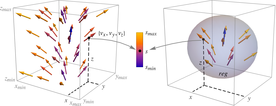
VectorPlot3D[…,{x,y,z}∈reg]
takes the variables {x,y,z} to be in the geometric region reg.
Details and Options
- VectorPlot3D is also known as field plot, quiver plot and direction plot.
- VectorPlot3D displays a vector field by drawing arrows normalized to a fixed length. The arrows are colored by default according to the magnitude
 of the vector field.
 - The plot visualizes the set
 .
. - VectorPlot3D by default shows vectors from the vector field at a specified grid of 3D positions.
- VectorPlot3D omits any arrows for which the vi etc. do not evaluate to real numbers.
- The region reg can be any RegionQ object in 3D.
- VectorPlot3D treats the variables x, y and z as local, effectively using Block.
- VectorPlot3D has attribute HoldAll and evaluates the vi etc. only after assigning specific numerical values to x, y and z. In some cases, it may be more efficient to use Evaluate to evaluate the vi etc. symbolically first.
- VectorPlot3D has the same options as Graphics3D, with the following additions and changes: [List of all options]
-
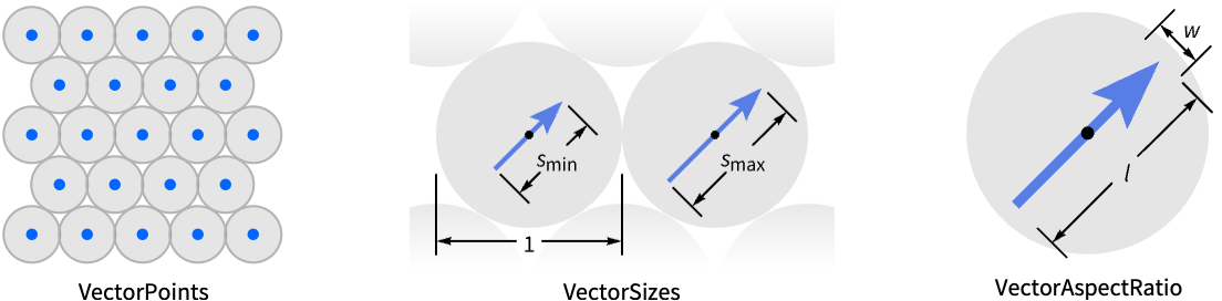
BoxRatios {1,1,1} ratio of height to width ClippingStyle Automatic how to display arrows outside the vector range EvaluationMonitor None expression to evaluate at every function evaluation Method Automatic methods to use for the plot PerformanceGoal $PerformanceGoal aspects of performance to try to optimize PlotLegends None legends to include PlotRange {Full,Full,Full} range of x, y, z values to include PlotRangePadding Automatic how much to pad the range of values PlotTheme $PlotTheme overall theme for the plot RegionBoundaryStyle Automatic how to style plot region boundaries RegionFunction (True&) determine what region to include ScalingFunctions None how to scale individual coordinates VectorAspectRatio Automatic width to length ratio for arrows VectorColorFunction Automatic how to color vectors VectorColorFunctionScaling True whether to scale the argument to VectorColorFunction VectorMarkers Automatic shape to use for arrows VectorPoints Automatic the number or placement of arrows VectorRange Automatic range of vector lengths to show VectorScaling None how to scale the sizes of arrows VectorSizes Automatic sizes of displayed arrows VectorStyle Automatic how to draw arrows WorkingPrecision MachinePrecision precision to use in internal computations - The individual arrows are scaled to fit inside bounding balls around each point.
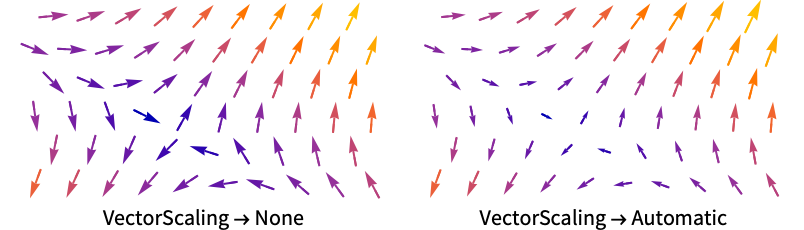
- VectorScaling scales the magnitudes of the vectors into the range of arrow sizes smin to smax given by VectorSizes.
- VectorScalingAutomatic will scale the arrow lengths depending on the vector magnitudes:
- Common markers include:
-
"Arrow3D" 3D arrow-shaped marker 
"Arrow" 2D arrow-shaped marker 
"Tube" tube segment aligned in the field direction 
"Segment" line segment aligned in the field direction - VectorColorFunctionNone will draw the arrows with the style specified by VectorStyle.
- The arguments supplied to functions in RegionFunction and VectorColorFunction are x, y, z, vx, vy, vz, Norm[{vx,vy,vz}].
- Possible settings for ScalingFunctions include:
-
{sx,sy,sz} scale x, y and z axes - Common built-in scaling functions s include:
-
"Log" 
log scale with automatic tick labeling "Log10" 
base-10 log scale with powers of 10 for ticks "SignedLog" 
log-like scale that includes 0 and negative numbers "Reverse" 
reverse the coordinate direction "Infinite" 
infinite scale
List of all options
Examples
open all close allBasic Examples (4)
VectorPlot3D[{x, y, z}, {x, -1, 1}, {y, -1, 1}, {z, -1, 1}]Include a legend for the vector magnitudes:
VectorPlot3D[{x, y, z}, {x, -1, 1}, {y, -1, 1}, {z, -1, 1}, PlotLegends -> Automatic]Use tube segments as markers to represent the vectors:
VectorPlot3D[{x, y, z}, {x, -1, 1}, {y, -1, 1}, {z, -1, 1}, VectorMarkers -> "Tube"]Plot a vector field inside the unit ball:
VectorPlot3D[{x, y, z}, {x, y, z}∈Ball[]]Scope (14)
Sampling (5)
Use Evaluate to evaluate the vector field symbolically before numeric assignment:
VectorPlot3D[Evaluate[D[Sin[x y z], {{x, y, z}}]], {x, -1, 1}, {y, -1, 1}, {z, -1, 1}, PlotRange -> All, VectorPoints -> 5]Plot vectors over specified regions:
VectorPlot3D[{x, y, z}, {x, -1, 1}, {y, -1, 1}, {z, -1, 1}, RegionFunction -> ((#1 #2 #3 > 0)&)]Plot a vector field with vectors placed with specified densities:
{VectorPlot3D[{x, y, z}, {x, -1, 1}, {y, -1, 1}, {z, -1, 1}, VectorPoints -> Coarse], VectorPlot3D[{x, y, z}, {x, -1, 1}, {y, -1, 1}, {z, -1, 1}, VectorPoints -> Fine]}Plot a field with arrows placed at random locations:
points = RandomReal[{-1, 1}, {500, 3}];VectorPlot3D[{x, y, z}, {x, -1, 1}, {y, -1, 1}, {z, -1, 1}, VectorPoints -> points]Plot multiple vector fields with different colors for each field:
VectorPlot3D[{{y, -x, z}, {x, y, z}}, {x, -1, 1}, {y, -1, 1}, {z, -1, 1}, VectorColorFunction -> None, VectorPoints -> 5]Presentation (9)
Plot a vector field with arrows scaled according to their magnitudes:
VectorPlot3D[{y, -x, z ^ 2}, {x, -1, 1}, {y, -1, 1}, {z, -1, 1}, VectorScaling -> Automatic]Use a single color for the arrows:
VectorPlot3D[{y, -x, z ^ 2}, {x, -1, 1}, {y, -1, 1}, {z, -1, 1}, VectorColorFunction -> None]VectorPlot3D[{y, -x, z}, {x, -1, 1}, {y, -1, 1}, {z, -1, 1}, PlotRange -> All, VectorPoints -> 5, VectorStyle -> "Arrow3D", VectorColorFunction -> "Rainbow"]Color and scale the vectors based on the norm of the field:
points = RandomReal[{-1, 1}, {500, 3}];VectorPlot3D[{x, y, z}, {x, -1, 1}, {y, -1, 1}, {z, -1, 1}, VectorScaling -> Automatic, VectorPoints -> points, PlotRange -> All, VectorColorFunction -> Hue]Plot a vector field with arrows of specified size:
Table[VectorPlot3D[{x, y, z}, {x, -1, 1}, {y, -1, 1}, {z, -1, 1}, VectorPoints -> 5, VectorSizes -> s, PlotLabel -> s], {s, {Small, Large, 2}}]Vary the arrow length and arrowhead size:
Table[VectorPlot3D[{x, y, z}, {x, -1, 1}, {y, -1, 1}, {z, -1, 1}, VectorPoints -> 5, VectorScaling -> Automatic, VectorSizes -> s, PlotLabel -> s], {s, {Small, Large, 2}}]points = Normalize /@ RandomReal[{-1, 1}, {250, 3}];VectorPlot3D[{{x, y, z}, {z, -y, x + y}}, {x, -1, 1}, {y, -1, 1}, {z, -1, 1}, VectorColorFunction -> None, VectorPoints -> points, PlotLegends -> {"one", "two"}]VectorPlot3D[{x, y, z}, {x, -1, 1}, {y, -1, 1}, {z, -1, 1}, PlotTheme -> "Marketing"]Use a log scale for the x axis:
VectorPlot3D[{x, y, z}, {x, 1, 100}, {y, 1, 10}, {z, 1, 10}, ScalingFunctions -> {"Log", None, None}]Reverse the y scale so it increases toward the bottom:
VectorPlot3D[{x, y, z}, {x, 1, 100}, {y, 1, 100}, {z, 1, 100}, ScalingFunctions -> {None, None, "Reverse"}]Options (94)
Axes (3)
By default, Axes are drawn for:
VectorPlot3D[{z, -y, x + y}, {x, -1, 1}, {y, -1, 1}, {z, -1, 1}]Use AxesFalse to turn off axes:
VectorPlot3D[{z, -y, x + y}, {x, -1, 1}, {y, -1, 1}, {z, -1, 1}, Axes -> False]Turn each axis on individually:
{VectorPlot3D[{z, -y, x + y}, {x, -1, 1}, {y, -1, 1}, {z, -1, 1}, Axes -> {True, False, False}], VectorPlot3D[{z, -y, x + y}, {x, -1, 1}, {y, -1, 1}, {z, -1, 1}, Axes -> {False, True, False}], VectorPlot3D[{z, -y, x + y}, {x, -1, 1}, {y, -1, 1}, {z, -1, 1}, Axes -> {False, False, True}]}AxesLabel (4)
No axes labels are drawn by default:
VectorPlot3D[{z, -y, x + y}, {x, -1, 1}, {y, -1, 1}, {z, -1, 1}]VectorPlot3D[{z, -y, x + y}, {x, -1, 1}, {y, -1, 1}, {z, -1, 1}, AxesLabel -> z]VectorPlot3D[{z, -y, x + y}, {x, -1, 1}, {y, -1, 1}, {z, -1, 1}, AxesLabel -> {x, y, z}]Use labels based on variables specified in VectorPlot3D:
VectorPlot3D[{z, -y, x + y}, {x, -1, 1}, {y, -1, 1}, {z, -1, 1}, AxesLabel -> Automatic]AxesOrigin (2)
AxesStyle (4)
Change the style for the axes:
VectorPlot3D[{z, -y, x + y}, {x, -1, 1}, {y, -1, 1}, {z, -1, 1}, AxesStyle -> StandardRed]Specify the style of each axis:
VectorPlot3D[{z, -y, x + y}, {x, -1, 1}, {y, -1, 1}, {z, -1, 1}, AxesStyle -> {{Thick, StandardBrown}, {Thick, StandardBlue}, {Thick, StandardGreen}}]Use different styles for the ticks and the axes:
VectorPlot3D[{z, -y, x + y}, {x, -1, 1}, {y, -1, 1}, {z, -1, 1}, AxesStyle -> StandardGreen, TicksStyle -> StandardGray]Use different styles for the labels and the axes:
VectorPlot3D[{z, -y, x + y}, {x, -1, 1}, {y, -1, 1}, {z, -1, 1}, AxesStyle -> StandardGreen, LabelStyle -> StandardGray]BoxRatios (2)
By default, BoxRatios is set to Automatic:
VectorPlot3D[{x, y, z}, {x, -1, 1}, {y, -1, 1}, {z, -1, 1}, BoxRatios -> Automatic]Make the height appear twice the width and length:
VectorPlot3D[{x, y, z}, {x, -1, 1}, {y, -1, 1}, {z, -1, 1}, BoxRatios -> {1, 1, 2}]EvaluationMonitor (2)
Show where the function is sampled:
ListPointPlot3D[Reap[VectorPlot3D[{x, y, z}, {x, -1, 1}, {y, -1, 1}, {z, -1, 1}, EvaluationMonitor :> Sow[{x, y, z}]]][[-1, 1]]]Count how many times the vector field function is evaluated:
Block[{k = 0}, VectorPlot3D[{x, y, z}, {x, -1, 1}, {y, -1, 1}, {z, -1, 1}, EvaluationMonitor :> k++];k]ImageSize (7)
Use named sizes such as Tiny, Small, Medium and Large:
{VectorPlot3D[{z, -y, x + y}, {x, -1, 1}, {y, -1, 1}, {z, -1, 1}, ImageSize -> Tiny], VectorPlot3D[{z, -y, x + y}, {x, -1, 1}, {y, -1, 1}, {z, -1, 1}, ImageSize -> Small]}Specify the width of the plot:
{VectorPlot3D[{z, -y, x + y}, {x, -1, 1}, {y, -1, 1}, {z, -1, 1}, ImageSize -> 150], VectorPlot3D[{z, -y, x + y}, {x, -1, 1}, {y, -1, 1}, {z, -1, 1}, AspectRatio -> 1.5, ImageSize -> 150]}Specify the height of the plot:
{VectorPlot3D[{z, -y, x + y}, {x, -1, 1}, {y, -1, 1}, {z, -1, 1}, ImageSize -> {Automatic, 150}], VectorPlot3D[{z, -y, x + y}, {x, -1, 1}, {y, -1, 1}, {z, -1, 1}, AspectRatio -> 2, ImageSize -> {Automatic, 150}]}Allow the width and height to be up to a certain size:
{VectorPlot3D[{z, -y, x + y}, {x, -1, 1}, {y, -1, 1}, {z, -1, 1}, ImageSize -> UpTo[200]], VectorPlot3D[{z, -y, x + y}, {x, -1, 1}, {y, -1, 1}, {z, -1, 1}, AspectRatio -> 2, ImageSize -> UpTo[200]]}Specify the width and height for a graphic, padding with space if necessary:
VectorPlot3D[{z, -y, x + y}, {x, -1, 1}, {y, -1, 1}, {z, -1, 1}, ImageSize -> {200, 300}, Background -> StandardBlue]Setting AspectRatioFull will fill the available space:
VectorPlot3D[{z, -y, x + y}, {x, -1, 1}, {y, -1, 1}, {z, -1, 1}, AspectRatio -> Full, ImageSize -> {200, 300}, Background -> StandardBlue]Use maximum sizes for the width and height:
{VectorPlot3D[{z, -y, x + y}, {x, -1, 1}, {y, -1, 1}, {z, -1, 1}, ImageSize -> {UpTo[150], UpTo[100]}], VectorPlot3D[{z, -y, x + y}, {x, -1, 1}, {y, -1, 1}, {z, -1, 1}, AspectRatio -> 2, ImageSize -> {UpTo[150], UpTo[100]}]}Use ImageSizeFull to fill the available space in an object:
Framed[Pane[VectorPlot3D[{z, -y, x + y}, {x, -1, 1}, {y, -1, 1}, {z, -1, 1}, ImageSize -> Full, Background -> StandardBlue], {200, 200}]]Specify the image size as a fraction of the available space:
Framed[Pane[VectorPlot3D[{z, -y, x + y}, {x, -1, 1}, {y, -1, 1}, {z, -1, 1}, AspectRatio -> Full, ImageSize -> {Scaled[0.5], Scaled[0.5]}, Background -> StandardBlue], {200, 200}]]PerformanceGoal (2)
Generate a higher-quality plot:
VectorPlot3D[{y, -x, z}, {x, -1, 1}, {y, -1, 1}, {z, -1, 1}, PerformanceGoal -> "Quality"]Emphasize performance, possibly at the cost of quality:
VectorPlot3D[{y, -x, z}, {x, -1, 1}, {y, -1, 1}, {z, -1, 1}, PerformanceGoal -> "Speed"]PlotLegends (5)
No legends are included by default:
VectorPlot3D[{z, -y, x + y}, {x, -1, 1}, {y, -1, 1}, {z, -1, 1}]Add a legend that indicates vector norms:
VectorPlot3D[{z, -y, x + y}, {x, -1, 1}, {y, -1, 1}, {z, -1, 1}, PlotLegends -> Automatic]Include a legend for two fields:
VectorPlot3D[{{x, y, z}, {z, -y, x + y}}, {x, -1, 1}, {y, -1, 1}, {z, -1, 1}, PlotLegends -> {"one", "two"}, VectorColorFunction -> None]Include the vector fields in the legend:
VectorPlot3D[{{x, y, z}, {z, -y, x + y}}, {x, -1, 1}, {y, -1, 1}, {z, -1, 1}, VectorColorFunction -> None, PlotLegends -> "Expressions"]Control the placement of the legend:
VectorPlot3D[{{x, y, z}, {z, -y, x + y}}, {x, -1, 1}, {y, -1, 1}, {z, -1, 1}, PlotLegends -> Placed[{"one", "two"}, Below],
	VectorColorFunction -> None]
PlotRange (9)
The full plot range is used by default:
VectorPlot3D[{x, y, z}, {x, -1, 1}, {y, -1, 1}, {z, -1, 1}, PlotRange -> Full]Use all points to compute the range:
VectorPlot3D[{x, y, z}, {x, -1, 1}, {y, -1, 1}, {z, -1, 1}, PlotRange -> All]Specify an explicit limit for ![]() ,
, ![]() , and
, and ![]() ranges:
ranges:
VectorPlot3D[{x, y, z}, {x, -1, 1}, {y, -1, 1}, {z, -1, 1}, PlotRange -> 2]VectorPlot3D[{x, y, z}, {x, -1, 1}, {y, -1, 1}, {z, -1, 1}, PlotRange -> {{-1, 2}, Automatic, Automatic}]Specify an explicit ![]() minimum range:
minimum range:
VectorPlot3D[{x, y, z}, {x, -1, 1}, {y, -1, 1}, {z, -1, 1}, PlotRange -> {{0, Full}, Automatic, Automatic}]VectorPlot3D[{x, y, z}, {x, -1, 1}, {y, -1, 1}, {z, -1, 1}, PlotRange -> {Full, {0, 2}, Automatic}]Specify an explicit ![]() maximum range:
maximum range:
VectorPlot3D[{x, y, z}, {x, -1, 1}, {y, -1, 1}, {z, -1, 1}, PlotRange -> {Full, {Full, 3}, Automatic}]VectorPlot3D[{x, y, z}, {x, -1, 1}, {y, -1, 1}, {z, -1, 1}, PlotRange -> {Full, Full, {-2, 2}}]Specify different ![]() ,
, ![]() , and
, and ![]() ranges:
ranges:
VectorPlot3D[{x, y, z}, {x, -1, 1}, {y, -1, 1}, {z, -1, 1}, PlotRange -> {{-2, 1.5}, {-1, 2}, {0, 1}}]PlotRangePadding (8)
Padding is computed automatically by default:
VectorPlot3D[{x, y, z}, {x, -1, 1}, {y, -1, 1}, {z, -1, 1}, PlotRangePadding -> Automatic]Specify no padding for all ![]() ,
, ![]() , and
, and ![]() ranges:
ranges:
VectorPlot3D[{x, y, z}, {x, -1, 1}, {y, -1, 1}, {z, -1, 1}, PlotRangePadding -> None]Specify an explicit padding for all ![]() ,
, ![]() , and
, and ![]() ranges:
ranges:
VectorPlot3D[{x, y, z}, {x, -1, 1}, {y, -1, 1}, {z, -1, 1}, PlotRangePadding -> 1]Add 10% padding to all ![]() ,
, ![]() , and
, and ![]() ranges:
ranges:
VectorPlot3D[{x, y, z}, {x, -1, 1}, {y, -1, 1}, {z, -1, 1}, PlotRangePadding -> Scaled[0.1]]Specify padding for ![]() and
and ![]() ranges:
ranges:
VectorPlot3D[{x, y, z}, {x, -1, 1}, {y, -1, 1}, {z, -1, 1}, PlotRangePadding -> {1, 0.5}]Specify different padding for ![]() ,
, ![]() , and
, and ![]() ranges:
ranges:
VectorPlot3D[{x, y, z}, {x, -1, 1}, {y, -1, 1}, {z, -1, 1}, PlotRangePadding -> {1, 0.5, 2}]Specify padding for the ![]() range:
range:
VectorPlot3D[{x, y, z}, {x, -1, 1}, {y, -1, 1}, {z, -1, 1}, PlotRangePadding -> {Automatic, Automatic, 2}]Use different padding forms for each dimension:
VectorPlot3D[{x, y, z}, {x, -1, 1}, {y, -1, 1}, {z, -1, 1}, PlotRangePadding -> {Automatic, Scaled[0.05], 2}]PlotTheme (2)
Use a theme with dense vector points and legends:
VectorPlot3D[{z, -y, x + y}, {x, 0, 1}, {y, 0, 1}, {z, 0, 1}, PlotTheme -> "Detailed"]Reduce the number of vector points:
VectorPlot3D[{z, -y, x + y}, {x, 0, 1}, {y, 0, 1}, {z, 0, 1}, PlotTheme -> "Detailed", VectorPoints -> Coarse]RegionBoundaryStyle (5)
Show the region defined by a region function:
VectorPlot3D[{x, y, z}, {x, -1, 1}, {y, -1, 1}, {z, -1, 1}, RegionFunction -> Function[{x, y, z}, Abs[x] + Abs[y] < 1]]Use None to not show the boundary:
VectorPlot3D[{x, y, z}, {x, -1, 1}, {y, -1, 1}, {z, -1, 1}, RegionFunction -> Function[{x, y, z}, Abs[x] + Abs[y] < 1], RegionBoundaryStyle -> None]Specify a style for the boundary:
VectorPlot3D[{x, y, z}, {x, -1, 1}, {y, -1, 1}, {z, -1, 1}, RegionFunction -> Function[{x, y, z}, Abs[x] + Abs[y] < 1], RegionBoundaryStyle -> Yellow]The boundaries of full rectangular regions are not shown:
VectorPlot3D[{x, y, z}, {x, -1, 1}, {y, -1, 1}, {z, -1, 1}]Specify a style for full rectangular regions:
VectorPlot3D[{x, y, z}, {x, -1, 1}, {y, -1, 1}, {z, -1, 1}, RegionBoundaryStyle -> Yellow]RegionFunction (3)
Plot vectors only over certain quadrants:
VectorPlot3D[{x, y, z}, {x, -1, 1}, {y, -1, 1}, {z, -1, 1}, RegionFunction -> ((#1 #2 #3 > 0)&)]Plot vectors only over regions where the field magnitude is above a given threshold:
VectorPlot3D[{x, y, z}, {x, -1, 1}, {y, -1, 1}, {z, -1, 1}, RegionFunction -> ((#7 > 1.4)&), VectorPoints -> 10]Use any logical combination of conditions:
VectorPlot3D[{x, y, z}, {x, -1, 1}, {y, -1, 1}, {z, -1, 1}, RegionFunction -> ((0.3 < #7 < 0.5 || 1.5 < #7 < 2)&), VectorPoints -> 10]ScalingFunctions (1)
Use a log scale for the x axis:
VectorPlot3D[{x, y, z}, {x, 1, 100}, {y, 1, 10}, {z, 1, 10}, ScalingFunctions -> {"Log", None, None}]Reverse the y scale so it increases toward the bottom:
VectorPlot3D[{x, y, z}, {x, 1, 100}, {y, 1, 100}, {z, 1, 100}, ScalingFunctions -> {None, None, "Reverse"}]Ticks (6)
Ticks are placed automatically in each plot:
VectorPlot3D[{x, y, z}, {x, -2, 2}, {y, -2, 2}, {z, -2, 2}]Use TicksNone to not draw any tick marks:
VectorPlot3D[{x, y, z}, {x, -2, 2}, {y, -2, 2}, {z, -2, 2}, Ticks -> None]Place tick marks at specific positions:
VectorPlot3D[{x, y, z}, {x, -2, 2}, {y, -2, 2}, {z, -2, 2}, Ticks -> {{-1.5, 0, 1.5}, {-1.5, 0, 1.5}, {-1.5, 0, 1.5}}]Draw tick marks at the specified positions with the specified labels:
VectorPlot3D[{x, y, z}, {x, -2, 2}, {y, -2, 2}, {z, -2, 2}, Ticks -> {{{-1.5, -a}, {0, 0}, {1.5, a}}, {{-1.5, -a}, {0, 0}, {1.5, a}}, {{-1.5, -a}, {0, 0}, {1.5, a}}}]Specify tick marks with scaled lengths:
VectorPlot3D[{x, y, z}, {x, -2, 2}, {y, -2, 2}, {z, -2, 2}, Ticks -> {{{-1.5, -a, .1}, {0, 0, .1}, {1.5, a, .1}}, {{-1.5, -a, .05}, {0, 0, .05}, {1.5, a, .05}}, {{-1.5, -a, .15}, {0, 0, .15}, {1.5, a, .15}}}]Customize each tick with position, length, labeling and styling:
VectorPlot3D[{x, y, z}, {x, -2, 2}, {y, -2, 2}, {z, -2, 2}, Ticks -> {{{-1.5, -a, .1, Directive[Red, Dashed, Thick]}, {0, 0, .1, Directive[Red, Dashed]}, {1.5, a, .1, Directive[Red]}}, {{-1.5, -a, .05, Directive[Blue, Dashed, Thick]}, {0, 0, .05, Directive[Blue, Dashed]}, {1.5, a, .05, Directive[Blue]}}, {{-1.5, -a, .15, Directive[Darker@Green, Dashed, Thick]}, {0, 0, .15, Directive[Darker@Green, Dashed]}, {1.5, a, .15, Directive[Darker@Green]}}}]TicksStyle (3)
By default, the ticks and tick labels use the same styles as the axis:
VectorPlot3D[{x, y, z}, {x, -2, 2}, {y, -2, 2}, {z, -2, 2}, AxesStyle -> StandardRed]Specify overall ticks style, including the tick labels:
VectorPlot3D[{x, y, z}, {x, -2, 2}, {y, -2, 2}, {z, -2, 2}, TicksStyle -> Directive[Bold, StandardRed]]Specify tick style for each of the axes:
VectorPlot3D[{x, y, z}, {x, -2, 2}, {y, -2, 2}, {z, -2, 2}, TicksStyle -> {Directive[StandardGray, Bold], Directive[Bold, StandardRed], Directive[Bold, StandardBlue]}]VectorAspectRatio (2)
The default aspect ratio for a vector marker is 0.3:
VectorPlot3D[{z y - z x(1 - x^2 - y^2)^2, -z x - z y(1 - x^2 - y^2)^2, z}, {x, -3, 3}, {y, -3, 3}, {z, -3, 3}, VectorAspectRatio -> 0.3]Decrease the relative width of a vector marker to its length:
VectorPlot3D[{z y - z x(1 - x^2 - y^2)^2, -z x - z y(1 - x^2 - y^2)^2, z}, {x, -3, 3}, {y, -3, 3}, {z, -3, 3}, VectorAspectRatio -> 0.2]VectorColorFunction (4)
Color the vectors according to their norm:
VectorPlot3D[{x, y, z}, {x, -1, 1}, {y, -1, 1}, {z, -1, 1}, VectorColorFunction -> Hue]Use any named color gradient from ColorData:
VectorPlot3D[{x, y, z}, {x, -1, 1}, {y, -1, 1}, {z, -1, 1}, VectorColorFunction -> "Rainbow"]Color the vectors according to their ![]() value:
value:
VectorPlot3D[{x, y, z}, {x, -1, 1}, {y, -1, 1}, {z, -1, 1}, VectorColorFunction -> Function[{x, y, z, vx, vy, vz, n}, ColorData["ThermometerColors"][x]]]Use VectorColorFunctionScalingFalse to get unscaled values:
VectorPlot3D[{x, y, z}, {x, -1, 1}, {y, -1, 1}, {z, -1, 1}, VectorColorFunction -> (ColorData[22][Round[#7]]&), VectorColorFunctionScaling -> False]VectorColorFunctionScaling (4)
By default, scaled values are used:
VectorPlot3D[{x, y, z}, {x, -1, 1}, {y, -1, 1}, {z, -1, 1}, VectorColorFunction -> Hue]Use VectorColorFunctionScalingFalse to get unscaled values:
VectorPlot3D[{x, y, z}, {x, -1, 1}, {y, -1, 1}, {z, -1, 1}, VectorColorFunction -> (ColorData[22][Round[#7]]&), VectorColorFunctionScaling -> False]Use unscaled coordinates in the ![]() direction and scaled coordinates in the
direction and scaled coordinates in the ![]() direction:
direction:
VectorPlot3D[{x, y, z}, {x, -1, 1}, {y, -1, 1}, {z, -1, 1}, VectorColorFunction -> Function[{x, y, z, vx, vy, vz, n}, Hue[x, y, 1]], VectorColorFunctionScaling -> {False, True}]Explicitly specify the scaling for each color function argument:
VectorPlot3D[{x, y, z}, {x, -1, 1}, {y, -1, 1}, {z, -1, 1}, VectorColorFunction -> (Hue[#7, #2, 1]&), VectorColorFunctionScaling -> {True, True, True, True, False}]VectorMarkers (3)
By default, 3D arrows are used:
VectorPlot3D[{x, y, z}, {x, -1, 1}, {y, -1, 1}, {z, -1, 1}]Table[VectorPlot3D[{x, y, z}, {x, -1, 1}, {y, -1, 1}, {z, -1, 1}, VectorMarkers -> m, PlotLabel -> m], {m, {"Tube", "Segment", "Arrow"}}]Use Placed to control the arrow placement relative to the vector points:
pts = Flatten[Table[{x, y, z}, {x, -1, 1}, {y, -1, 1}, {z, -1, 1}], 2];Table[Show[VectorPlot3D[{x, y, z}, {x, -1, 1}, {y, -1, 1}, {z, -1, 1}, VectorMarkers -> Placed["Arrow", pos], VectorPoints -> pts],
ListPointPlot3D[pts]], {pos, {"Start", "End"}}]VectorPoints (7)
Use automatically determined vector points:
VectorPlot3D[{x, y, z}, {x, -1, 1}, {y, -1, 1}, {z, -1, 1}, VectorPoints -> Automatic]Use symbolic names to specify the set of field vectors:
Table[VectorPlot3D[{x, y, z}, {x, -1, 1}, {y, -1, 1}, {z, -1, 1}, PlotLabel -> k, VectorPoints -> k], {k, {Fine, Coarse}}]Create a regular grid of field vectors with the same number of arrows for ![]() ,
, ![]() , and
, and ![]() :
:
VectorPlot3D[{x, y, z}, {x, -1, 1}, {y, -1, 1}, {z, -1, 1}, VectorPoints -> 5]Create a regular grid of field vectors with a different number of arrows for ![]() ,
, ![]() , and
, and ![]() :
:
VectorPlot3D[{x, y, z}, {x, -1, 1}, {y, -1, 1}, {z, -1, 1}, VectorPoints -> {4, 7, 9}]Specify a list of points for showing field vectors:
VectorPlot3D[{x, y, z}, {x, -1, 1}, {y, -1, 1}, {z, -1, 1}, VectorPoints -> RandomReal[{-1, 1}, {300, 3}]]Use a different number of field vectors on a packed grid:
Table[VectorPlot3D[{x, y, z}, {x, -1, 1}, {y, -1, 1}, {z, -1, 1}, PlotLabel -> n, VectorPoints -> n], {n, 4, 10, 3}]The location for vectors is given in the middle of the drawn vector:
points = {{-1, -1, -1}, {-1, 1, 1}, {1, -1, -1}, {1, 1, 1}};Show[VectorPlot3D[{x, y, z}, {x, -2, 2}, {y, -2, 2}, {z, -2, 2}, VectorPoints -> points, PlotRange -> 2], Graphics3D[{Red, Sphere[points, 0.15]}]]Start the vectors at the points:
Show[VectorPlot3D[{x, y, z}, {x, -2, 2}, {y, -2, 2}, {z, -2, 2}, VectorPoints -> points, PlotRange -> 2, VectorMarkers -> "Start"], Graphics3D[{Red, Sphere[points, 0.15]}]]VectorRange (4)
The clipping of vectors with very small or very large magnitudes is done automatically:
VectorPlot3D[({x, y, z}/Norm[{x, y, z}]^3), {x, -3, 3}, {y, -3, 3}, {z, -3, 3}, VectorRange -> Automatic]Specify the range of vector norms:
VectorPlot3D[({x, y, z}/Norm[{x, y, z}]^3), {x, -3, 3}, {y, -3, 3}, {z, -3, 3}, VectorRange -> {0.1, 2}]VectorPlot3D[({x, y, z}/Norm[{x, y, z}]^3), {x, -3, 3}, {y, -3, 3}, {z, -3, 3}, VectorRange -> {0.1, 2}, ClippingStyle -> None]VectorPlot3D[({x, y, z}/Norm[{x, y, z}]^3), {x, -3, 3}, {y, -3, 3}, {z, -3, 3}, VectorRange -> All]VectorStyle (2)
VectorColorFunction takes precedence over colors in VectorStyle:
VectorPlot3D[{x, y, z}, {x, -1, 1}, {y, -1, 1}, {z, -1, 1}, VectorStyle -> Red]Use VectorColorFunction→None to specify colors with VectorStyle:
VectorPlot3D[{x, y, z}, {x, -1, 1}, {y, -1, 1}, {z, -1, 1}, VectorStyle -> StandardRed, VectorColorFunction -> None]Applications (1)
An electrostatic potential built from a collection of point charges ![]() at positions
at positions ![]() :
:
electroStaticPotential[q_, p_, r_] := Sum[ (q[[i]]/Norm[r - p[[i]]]), {i, Length[q]}]electroStaticPotential[{Subscript[q, 1], Subscript[q, 2]}, {{Subscript[x, 1], Subscript[y, 1], Subscript[z, 1]}, {Subscript[x, 2], Subscript[y, 2], Subscript[z, 2]}}, {x, y, z}]//TraditionalFormAn electric field between two charges ![]() and
and ![]() :
:
electricField[{q1_, q2_}, {{x1_, y1_, z1_}, {x2_, y2_, z2_}}] = -D[electroStaticPotential[{q1, q2}, {{x1, y1, z1}, {x2, y2, z2}}, {x, y, z}], {{x, y, z}}] /. Derivative[1][Abs][x_] :> (x/Sqrt[x^2]);The electrostatic potential between two charges ![]() and
and ![]() :
:
c = ContourPlot3D[Evaluate[electroStaticPotential[{1, -1}, {{-1, 0, 0}, {1, 0, 0}}, {x, y, z}]], {x, -6, 6}, {y, 0, 4}, {z, -4, 4}, Contours -> {-0.75, -0.25, -0.1, 0, 0.1, 0.25, 0.75}, ContourStyle -> Table[Hue[i / 7, 1, 1, 0.5], {i, 0, 6}], Mesh -> None]The electric field between two charges ![]() and
and ![]() :
:
v = VectorPlot3D[electricField[{1, -1}, {{-1, 0, 0}, {1, 0, 0}}], {x, -6, 6}, {y, 0, 4}, {z, -4, 4}, VectorPoints -> 5]Show[v, c]Properties & Relations (14)
Use ListVectorPlot3D to visualize data:
vectors = Table[{x, y, z}, {x, -1, 1, .1}, {y, -1, 1, .1}, {z, -1, 1, .1}];ListVectorPlot3D[vectors]Plot vectors along surfaces with SliceVectorPlot3D:
SliceVectorPlot3D[{x, y, z}, {x, -1, 1}, {y, -1, 1}, {z, -1, 1}]Plot data vectors on surfaces with ListSliceVectorPlot3D:
data = Table[{z, x, x + y}, {x, -1, 1}, {y, -1, 1}, {z, -1, 1}];ListSliceVectorPlot3D[data, "CenterPlanes"]Use StreamPlot3D to plot streamlines for a 3D vector field:
StreamPlot3D[{z, -x, y}, {x, -2, 2}, {y, -2, 2}, {z, -2, 2}]Use ListStreamPlot3D to plot with data:
data = Table[{z, -x, y}, {x, -2, 2}, {y, -2, 2}, {z, -2, 2}];ListStreamPlot3D[data]Use VectorDisplacementPlot to visualize the effect of a displacement vector field on a specified region:
VectorDisplacementPlot[{-1 - x ^ 2 + y, 1 + x - y ^ 2}, {x, y}∈Annulus[], VectorPoints -> Automatic]Use ListVectorDisplacementPlot to visualize the effect of displacement field data on a region:
data = Table[{{x, y}, {x + y, 1 + x - y}}, {x, -3, 3, 0.2}, {y, -3, 3, 0.2}];ListVectorDisplacementPlot[data, Polygon[{{3, 3}, {0, 1}, {-3, 3}, {-3, -3}, {0, -1}, {3, -3}}], VectorPoints -> Automatic]Use VectorDisplacementPlot3D to visualize the effect of a displacement vector field on a specified 3D region:
VectorDisplacementPlot3D[{-y, x, x + z}, {x, -2, 2}, {y, -2, 2}, {z, -2, 2}, VectorPoints -> "Boundary"]Use ListVectorDisplacementPlot3D to visualize the effect of 3D displacement vector field data on a specified region:
data = Table[{{x, y, z}, {-y, x, x + z}}, {x, -2, 2}, {y, -2, 2}, {z, -2, 2}];ListVectorDisplacementPlot3D[data, VectorPoints -> "Boundary"]Use VectorPlot for plotting 2D vectors:
VectorPlot[{y, -x}, {x, -2, 2}, {y, -2, 2}]Use ListVectorPlot to plot with data:
data = Table[{y, -x}, {x, -2, 2}, {y, -2, 2}];ListVectorPlot[data]Use StreamPlot to plot with streamlines instead of vectors:
StreamPlot[{-1 - x ^ 2 + y, 1 + x - y ^ 2}, {x, -3, 3}, {y, -3, 3}]data = Table[{-1 - x ^ 2 + y, 1 + x - y ^ 2}, {x, -3, 3, 0.1}, {y, -3, 3, 0.1}];ListStreamPlot[data]Use VectorDensityPlot to add a density plot of the scalar field:
VectorDensityPlot[{-1 - x ^ 2 + y, 1 + x - y ^ 2}, {x, -3, 3}, {y, -3, 3}]Use StreamDensityPlot to plot streamlines instead of vectors:
StreamDensityPlot[{-1 - x ^ 2 + y, 1 + x - y ^ 2}, {x, -3, 3}, {y, -3, 3}]Use ListVectorDensityPlot or ListStreamDensityPlot for plotting data:
data = Table[{{x, y} = RandomReal[{-1.5, 1.5}, {2}], {{y, x - x ^ 3}, Abs[x + y]}}, {300}];{ListVectorDensityPlot[data], ListStreamDensityPlot[data]}Use LineIntegralConvolutionPlot to plot the line integral convolution of a vector field:
LineIntegralConvolutionPlot[{-1 - x ^ 2 + y, 1 + x - y ^ 2}, {x, -3, 3}, {y, -3, 3}]Plot a complex function as a vector field:
ComplexVectorPlot[z + 1 / z, {z, 2}]Plot streams instead of vectors with ComplexStreamPlot:
ComplexStreamPlot[z^2 + 1, {z, 2}]Use GeoVectorPlot to generate a vector plot over the Earth:
coords = Flatten[Table[{lat, long}, {long, -180, 180, 30}, {lat, -75, 75, 15}], 1];vects = Table[{RandomReal[], Quantity[RandomReal[{0, 360}], "AngularDegrees"]}, {Length[coords]}];GeoVectorPlot[GeoVector[GeoPosition[coords] -> vects]]Use GeoStreamPlot to use streams instead of vectors:
GeoStreamPlot[GeoVector[GeoPosition[coords] -> vects]]Text
Wolfram Research (2008), VectorPlot3D, Wolfram Language function, https://reference.wolfram.com/language/ref/VectorPlot3D.html (updated 2022).
CMS
Wolfram Language. 2008. "VectorPlot3D." Wolfram Language & System Documentation Center. Wolfram Research. Last Modified 2022. https://reference.wolfram.com/language/ref/VectorPlot3D.html.
APA
Wolfram Language. (2008). VectorPlot3D. Wolfram Language & System Documentation Center. Retrieved from https://reference.wolfram.com/language/ref/VectorPlot3D.html