



SliceContourPlot3D
SliceContourPlot3D[f,surf,{x,xmin,xmax},{y,ymin,ymax},{z,zmin,zmax}]
在切片曲面 surf 上,生成以 x、y、z 为函数的 f 的等高线图.
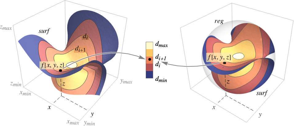
SliceContourPlot3D[f,surf,{x,y,z}∈reg]
将切片曲面的范围限制在区域 reg 内.
SliceContourPlot3D[f,{surf1,surf2,…},…]
在多个切片上生成等高线图.
更多信息和选项
- SliceContourPlot3D 在曲面 surf 上构建等值线,对应于 f[x,y,z] 的值为常数 d1、d2 等的水平集. 默认情况下,曲线间的区域被着色,以便更容易识别值介于 di 和 di+1 之间的区域.
- 函数可视化区域
 .
- 可以给出以下基本切片曲面 surfi:
-
Automatic 自动确定切片曲面 
"CenterPlanes" 过中心点的坐标平面 
"BackPlanes" 图形后面的坐标平面 
"XStackedPlanes" 沿  轴叠放的坐标平面

"YStackedPlanes" 沿  轴叠放的坐标平面

"ZStackedPlanes" 沿  轴叠放的坐标平面

"DiagonalStackedPlanes" 沿对角线叠放的坐标平面 
"CenterSphere" 位于中心的球面 
"CenterCutSphere" 切去楔形块的球面 
"CenterCutBox" 八分之一被切掉的盒子 - SliceContourPlot3D[f,{x,xmin,xmax},…] 等价于 SliceContourPlot3D[f,Automatic,{x,xmin,xmax},…] 等.
- 以下参数化可以用于基本切片曲面:
-
{"XStackedPlanes",n}, 生成 n 个等间隔平面 {"XStackedPlanes",{x1,x2,…}} 生成平面 
{"CenterCutSphere",ϕopen} 正对视点处切去角 ϕopen {"CenterCutSphere",ϕopen,ϕcenter} 以  平面上的 ϕcenter 为中心角切去角 ϕopen
- "YStackedPlanes"、"ZStackedPlanes" 和 "XStackedPlanes" 的规范一样,在“范围”下面的例子中会展示更多的用法.
- 可以使用下列常见的切片曲面 surfi:
-
expr0 以 x、y 和 z 表示的隐方程,如 x y z-10 surfaceregion 三维空间中的二维区域,如 Hyperplane volumeregion 三维空间中的三维区域,其中 surfi 为边界曲面,如 Cuboid - 可将下列封装用于切片曲面 surfi:
-
Annotation[surf,label] 提供注释 Button[surf,action] 定义当曲面被点击时应执行的操作 EventHandler[surf,…] 为曲面定义通用事件处理程序 (general event handler) Hyperlink[surf,uri] 将曲面设置为超链接 PopupWindow[surf,cont] 为曲面添加弹出窗口 StatusArea[surf,label] 当鼠标悬停在曲面处时,在状态栏中显示的内容 Tooltip[surf,label] 为曲面添加任意提示条 - SliceContourPlot3D 与 Graphics3D 的选项相同,不同之处和更多选项如下所示: [所有选项的列表]
-
Axes True 是否绘制坐标轴 BoundaryStyle Automatic 如何设计曲面边界 BoxRatios {1,1,1} 三维边界盒的比例 ClippingStyle None 如何绘制用 PlotRange 修剪过的值 ColorFunction Automatic 如何为图上色 ColorFunctionScaling True 是否缩放传递给 ColorFunction 的参数 Contours Automatic 在每个曲面上显示多少个或显示什么样的等高线 ContourShading Automatic 如何为等高线间的区域做明暗处理 ContourStyle Automatic 等高线的样式 PerformanceGoal $PerformanceGoal 优化的目标 PlotLegends None 颜色梯度的图例 PlotPoints Automatic 每个方向上函数 f 和切片曲面 surfi 的初始样本数 PlotRange {Full,Full,Full,Automatic} 函数 f 的值域或要包括的其他值 PlotTheme $PlotTheme 图的整体主题 RegionFunction (True&) 如何决定是否要包括某个点 ScalingFunctions None 怎样缩放个别坐标 TargetUnits Automatic 想要使用的单位 WorkingPrecision MachinePrecision 内部计算时使用的精度 - 默认情况下,传递给 ColorFunction 的是经过缩放的 f 值.
- 默认情况下,RegionFunction 的变量由 x、y、z 和 f 提供.
- ScalingFunctions 的可能设置包括:
-
sf 缩放 f 等值线的值 {sx,sy,sz} 缩放 x、y 和 z 坐标轴 {sx,sy,sz,sf} 缩放 x、y 和 z 坐标轴以及 f 等值线的值 - 常见内置缩放函数 s 包括:
-
"Log" 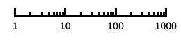
对数刻度,自动进行标记 "Log10" 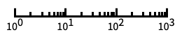
以 10 为底的对数刻度,用 10 的幂进行标记 "SignedLog" 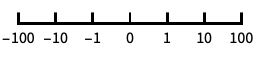
类似对数的刻度,包含 0 和负数 "Reverse" 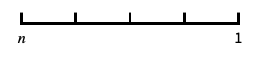
反转坐标的方向 "Infinite" 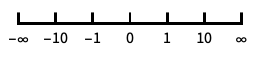
无穷刻度
所有选项的列表
范例
打开所有单元 关闭所有单元基本范例 (2)


范围 (24)
曲面 (9)
Table[SliceContourPlot3D[Sin[x] + y ^ 2 - z ^ 3, sl, {x, -1, 1}, {y, -1, 1}, {z, -1, 1}, PlotLabel -> sl], {sl, {"CenterPlanes", "BackPlanes", "DiagonalStackedPlanes"}}]Table[SliceContourPlot3D[Sin[x] + y ^ 2 - z ^ 3, sl, {x, -1, 1}, {y, -1, 1}, {z, -1, 1}, PlotLabel -> sl], {sl, {"XStackedPlanes", "YStackedPlanes", "ZStackedPlanes"}}]Table[SliceContourPlot3D[Sin[x] + y ^ 2 - z ^ 3, sl, {x, -1, 1}, {y, -1, 1}, {z, -1, 1}, PlotLabel -> sl], {sl, {"CenterSphere", "CenterCutSphere", "CenterCutBox"}}]SliceContourPlot3D[x + y + z, HalfPlane[{{0, 0, 0}, {1, 0, 0}}, {0, 1, 1}], {x, -1, 1}, {y, -1, 1}, {z, -1, 1}]在基本几何体(volume primitive)上绘制等高线图相当于在 RegionBoundary[reg] 上绘制:
SliceContourPlot3D[x + y + z, Cylinder[], {x, -1, 1}, {y, -1, 1}, {z, -1, 1}]
SliceContourPlot3D[Sin[x y z], x ^ 3 + y ^ 2 - z ^ 2 == 0, {x, -2, 2}, {y, -2, 2}, {z, -2, 2}]SliceContourPlot3D[Sin[x y z], {Cylinder[], "BackPlanes"}, {x, -2, 2}, {y, -2, 2}, {z, -2, 2}, Contours -> 3]SliceContourPlot3D[x + y + z, {"XStackedPlanes", 7}, {x, -2, 2}, {y, -2, 2}, {z, -2, 2}]SliceContourPlot3D[Sin[x y z], {"CenterCutSphere", 2Pi / 3}, {x, -2, 2}, {y, -2, 2}, {z, -2, 2}]抽样 (4)
使用 Contours 指定等高线的数量:
SliceContourPlot3D[x + y + z, "BackPlanes", {x, -2, 2}, {y, -2, 2}, {z, -2, 2}, Contours -> 5]
SliceContourPlot3D[x + y + z, "BackPlanes", {x, -2, 2}, {y, -2, 2}, {z, -2, 2}, Contours -> {-1, 0, 1}]SliceContourPlot3D[Sqrt[x y z], "CenterSphere", {x, -1, 1}, {y, -1, 1}, {z, -1, 1}]用 RegionFunction 来显示被遮挡的切片:
SliceContourPlot3D[x ^ 2 + y ^ 2 + z ^ 2, "ZStackedPlanes", {x, -2, 2}, {y, -2, 2}, {z, -2, 2}, RegionFunction -> Function[{x, y, z}, x < 0 || y > 0]]可以用包含 Cone 的区域来指定值域:
SliceContourPlot3D[x + y + z, "CenterPlanes", {x, y, z}∈Cone[]]一个含有 ImplicitRegion 的公式区域(formula region):
ℛ = ImplicitRegion[(x ^ 2 + (9 / 4)y ^ 2 + z ^ 2 - 1) ^ 3 - x ^ 2z ^ 3 - (9 / 80)y ^ 2z ^ 3 <= 0, {{x, -1.2, 1.2}, {y, -0.7, 0.7}, {z, -1, 1.3}}];SliceContourPlot3D[x + y + z, "CenterPlanes", {x, y, z}∈ℛ]一个含有 BoundaryMeshRegion 的基于网格的区域:
ℛ = ConvexHullMesh[RandomReal[1, {25, 3}]]SliceContourPlot3D[x + y + z, "CenterPlanes", {x, y, z}∈ℛ]演示 (11)
使用 PlotTheme 对整体样式进行配置:
Table[SliceContourPlot3D[x ^ 2 + y ^ 2 + z ^ 2, "CenterPlanes", {x, -1, 1}, {y, -1, 1}, {z, -1, 1}, PlotLabel -> t, PlotTheme -> t], {t, {"Minimal", "Scientific", "Marketing"}}]用 PlotLegends 显示不同数值对应的颜色:
SliceContourPlot3D[x ^ 2 + y ^ 2 + z ^ 2, "CenterPlanes", {x, -1, 1}, {y, -1, 1}, {z, -1, 1}, PlotLegends -> Automatic]用 Axes 控制坐标轴的显示:
Table[SliceContourPlot3D[x + y + z, "CenterPlanes", {x, -2, 2}, {y, -2, 2}, {z, -2, 2}, PlotLabel -> a, Axes -> a], {a, {True, False, {True, False, True}}}]可使用 AxesLabel 为坐标轴添加标签,使用 PlotLabel 为整个图添加标签:
SliceContourPlot3D[x ^ 2 + y ^ 2 + z ^ 2, "CenterPlanes", {x, -2, 2}, {y, -2, 2}, {z, -2, 2}, Ticks -> None, AxesLabel -> {x, y, z}, PlotLabel -> x ^ 2 + y ^ 2 + z ^ 2]用 ColorFunction 根据函数值为图上色:
Table[SliceContourPlot3D[Sin[3x y z], "ZStackedPlanes", {x, -1, 1}, {y, -1, 1}, {z, -1, 1}, PlotLabel -> c, ColorFunction -> c], {c, {Hue, "BlueGreenYellow"}}]用 ContourShading 为等高线间的区域设计样式:
SliceContourPlot3D[Exp[-(x ^ 2 + y ^ 2 + z ^ 2)], "CenterPlanes", {x, -1, 1}, {y, -1, 1}, {z, -1, 1}, Contours -> 9, BoundaryStyle -> None, ContourShading -> {Orange, None, Blue}]用 ContourStyle 为等高线设计样式:
SliceContourPlot3D[x ^ 4 + y ^ 4 + z ^ 4 - x ^ 2 - y ^ 2 - z ^ 2, "CenterSphere", {x, -1, 1}, {y, -1, 1}, {z, -1, 1}, ContourStyle -> Dotted]用 BoundaryStyle 为切片曲面边界设计样式:
SliceContourPlot3D[Exp[-(x ^ 2 + y ^ 2 + z ^ 2)], "CenterPlanes", {x, -2, 2}, {y, -2, 2}, {z, -2, 2}, BoundaryStyle -> Gray]TargetUnits 指定在可视化时使用哪个单位:
SliceContourPlot3D[Quantity[-(x ^ 2 + y ^ 2 + z ^ 2), "kg/m^3"], "CenterPlanes", {x, -2, 2}, {y, -2, 2}, {z, -2, 2}, AxesLabel -> Automatic, PlotLegends -> Automatic, TargetUnits -> {"Feet", "Feet", "Feet", "g/ft^3"}]
SliceContourPlot3D[x + y + z, {x, 1, 100}, {y, 1, 100}, {z, 1, 100}, ScalingFunctions -> {"Log", None, None}]
SliceContourPlot3D[x + y + z, {x, 1, 100}, {y, 1, 100}, {z, 1, 100}, ScalingFunctions -> {None, None, "Reverse"}]选项 (71)
Axes (3)
SliceContourPlot3D[-(x ^ 2 + y ^ 2 + z ^ 2), "CenterPlanes", {x, -2, 2}, {y, -2, 2}, {z, -2, 2}]SliceContourPlot3D[-(x ^ 2 + y ^ 2 + z ^ 2), "CenterPlanes", {x, -2, 2}, {y, -2, 2}, {z, -2, 2}, Axes -> False]{SliceContourPlot3D[-(x ^ 2 + y ^ 2 + z ^ 2), "CenterPlanes", {x, -2, 2}, {y, -2, 2}, {z, -2, 2}, Axes -> {False, False, True}], SliceContourPlot3D[-(x ^ 2 + y ^ 2 + z ^ 2), "CenterPlanes", {x, -2, 2}, {y, -2, 2}, {z, -2, 2}, Axes -> {False, True, False}], SliceContourPlot3D[-(x ^ 2 + y ^ 2 + z ^ 2), "CenterPlanes", {x, -2, 2}, {y, -2, 2}, {z, -2, 2}, Axes -> {True, False, False}]}AxesLabel (4)
SliceContourPlot3D[-(x ^ 2 + y ^ 2 + z ^ 2), "CenterPlanes", {x, -2, 2}, {y, -2, 2}, {z, -2, 2}]
SliceContourPlot3D[-(x ^ 2 + y ^ 2 + z ^ 2), "CenterPlanes", {x, -2, 2}, {y, -2, 2}, {z, -2, 2}, AxesLabel -> "height"]SliceContourPlot3D[-(x ^ 2 + y ^ 2 + z ^ 2), "CenterPlanes", {x, -2, 2}, {y, -2, 2}, {z, -2, 2}, AxesLabel -> {"width", "depth", "height"}]使用的标签基于在 SliceContourPlot3D 中指定的变量:
SliceContourPlot3D[-(x ^ 2 + y ^ 2 + z ^ 2), "CenterPlanes", {x, -2, 2}, {y, -2, 2}, {z, -2, 2}, AxesLabel -> Automatic]AxesOrigin (2)
AxesStyle (3)
SliceContourPlot3D[-(x ^ 2 + y ^ 2 + z ^ 2), "CenterPlanes", {x, -2, 2}, {y, -2, 2}, {z, -2, 2}, AxesStyle -> Red]SliceContourPlot3D[-(x ^ 2 + y ^ 2 + z ^ 2), "CenterPlanes", {x, -2, 2}, {y, -2, 2}, {z, -2, 2}, AxesStyle -> {{Thick, Brown}, {Thick, Blue}, {Thick, Green}}]SliceContourPlot3D[-(x ^ 2 + y ^ 2 + z ^ 2), "CenterPlanes", {x, -2, 2}, {y, -2, 2}, {z, -2, 2}, AxesStyle -> Green, TicksStyle -> Blue]BoundaryStyle (1)
使用 BoundaryStyle 为切片曲面边界设计样式:
SliceContourPlot3D[-(x ^ 2 + y ^ 2 + z ^ 2), "CenterPlanes", {x, -2, 2}, {y, -2, 2}, {z, -2, 2}, BoundaryStyle -> Gray]BoxRatios (3)
SliceContourPlot3D[x y z, "CenterSphere", {x, 0, 1}, {y, 0, 1}, {z, -1, 2}]使用 BoxRatios->Automatic 来显示三维坐标本来的比例:
SliceContourPlot3D[x y z, "CenterSphere", {x, 0, 1}, {y, 0, 1}, {z, -1, 2}, BoxRatios -> Automatic]SliceContourPlot3D[x y z, "CenterSphere", {x, 0, 1}, {y, 0, 1}, {z, -1, 2}, BoxRatios -> {1, 2, 2}]ClippingStyle (2)
SliceContourPlot3D[Exp[-(x ^ 2 + y ^ 2 + z ^ 2)], "CenterPlanes", {x, -2, 2}, {y, -2, 2}, {z, -2, 2}, PlotRange -> {0.09, 0.72}, ClippingStyle -> {Gray, Green}]用 None 去掉剪切区域:
SliceContourPlot3D[Exp[-(x ^ 2 + y ^ 2 + z ^ 2)], "CenterPlanes", {x, -2, 2}, {y, -2, 2}, {z, -2, 2}, PlotRange -> {0.09, 0.72}, ClippingStyle -> None]ColorFunction (3)

SliceContourPlot3D[x + y z, "ZStackedPlanes", {x, -1, 1}, {y, -1, 1}, {z, -1, 1}, ColorFunction -> Hue]SliceContourPlot3D[x ^ 2 + y ^ 2 + z ^ 2, "CenterPlanes", {x, -2, 2}, {y, -2, 2}, {z, -2, 2}, ColorFunction -> "IslandColors"]
SliceContourPlot3D[Sin[2 x y z], "ZStackedPlanes", {x, -2, 2}, {y, -2, 2}, {z, -2, 2}, ColorFunction -> Function[f, If[f < 0, Red, Green]],
	ColorFunctionScaling -> False, Contours -> 3]
ColorFunctionScaling (2)
SliceContourPlot3D[x y z, "BackPlanes", {x, -2, 2}, {y, -2, 2}, {z, -2, 2}, ColorFunction -> Hue]用 ColorFunctionScalingFalse 来得到未经缩放的值:
SliceContourPlot3D[x y z, "BackPlanes", {x, -2, 2}, {y, -2, 2}, {z, -2, 2}, ColorFunction -> (If[# <= 0, Red, Green]&), ColorFunctionScaling -> False]Contours (4)
SliceContourPlot3D[x ^ 3 + y ^ 2 - z ^ 2, "BackPlanes", {x, -2, 2}, {y, -2, 2}, {z, -2, 2}, Contours -> 5]SliceContourPlot3D[x ^ 3 + y ^ 2 - z ^ 2, "BackPlanes", {x, -2, 2}, {y, -2, 2}, {z, -2, 2}, Contours -> Automatic]SliceContourPlot3D[x ^ 3 + y ^ 2 - z ^ 2, "BackPlanes", {x, -2, 2}, {y, -2, 2}, {z, -2, 2}, Contours -> {-1, 1}]SliceContourPlot3D[x ^ 3 + y ^ 2 - z ^ 2, "BackPlanes", {x, -2, 2}, {y, -2, 2}, {z, -2, 2}, Contours -> {{-1, Green}, {1, Dashed}}]ContourStyle (1)
ContourShading (4)
ContourShadingAutomatic 根据 ColorFunction 计算等高线区域的色调:
SliceContourPlot3D[Exp[-(x ^ 2 + y ^ 2 + z ^ 2)], "CenterPlanes", {x, -1, 1}, {y, -1, 1}, {z, -1, 1}, Contours -> 9, BoundaryStyle -> None, ContourShading -> Automatic, ColorFunction -> "BrightBands"]SliceContourPlot3D[Exp[-(x ^ 2 + y ^ 2 + z ^ 2)], "CenterPlanes", {x, -1, 1}, {y, -1, 1}, {z, -1, 1}, Contours -> 9, BoundaryStyle -> None, ContourShading -> {Orange, Blue}]SliceContourPlot3D[Exp[-(x ^ 2 + y ^ 2 + z ^ 2)], "CenterPlanes", {x, -1, 1}, {y, -1, 1}, {z, -1, 1}, Contours -> 9, BoundaryStyle -> None, ContourShading -> {Orange, None, Blue}]SliceContourPlot3D[Exp[-(x ^ 2 + y ^ 2 + z ^ 2)], "CenterPlanes", {x, -1, 1}, {y, -1, 1}, {z, -1, 1}, Contours -> 9, BoundaryStyle -> None, ContourShading -> None]ImageSize (7)
使用命名尺寸,例如 Tiny、Small、Medium 和 Large:
{SliceContourPlot3D[-(x ^ 2 + y ^ 2 + z ^ 2), "CenterPlanes", {x, -2, 2}, {y, -2, 2}, {z, -2, 2}, ImageSize -> Tiny], SliceContourPlot3D[-(x ^ 2 + y ^ 2 + z ^ 2), "CenterPlanes", {x, -2, 2}, {y, -2, 2}, {z, -2, 2}, ImageSize -> Small]}{SliceContourPlot3D[-(x ^ 2 + y ^ 2 + z ^ 2), "CenterPlanes", {x, -2, 2}, {y, -2, 2}, {z, -2, 2}, ImageSize -> 150], SliceContourPlot3D[-(x ^ 2 + y ^ 2 + z ^ 2), "CenterPlanes", {x, -2, 2}, {y, -2, 2}, {z, -2, 2}, AspectRatio -> 1.5, ImageSize -> 150]}{SliceContourPlot3D[-(x ^ 2 + y ^ 2 + z ^ 2), "CenterPlanes", {x, -2, 2}, {y, -2, 2}, {z, -2, 2}, ImageSize -> {Automatic, 150}], SliceContourPlot3D[-(x ^ 2 + y ^ 2 + z ^ 2), "CenterPlanes", {x, -2, 2}, {y, -2, 2}, {z, -2, 2}, AspectRatio -> 2, ImageSize -> {Automatic, 150}]}{SliceContourPlot3D[-(x ^ 2 + y ^ 2 + z ^ 2), "CenterPlanes", {x, -2, 2}, {y, -2, 2}, {z, -2, 2}, ImageSize -> UpTo[200]], SliceContourPlot3D[-(x ^ 2 + y ^ 2 + z ^ 2), "CenterPlanes", {x, -2, 2}, {y, -2, 2}, {z, -2, 2}, AspectRatio -> 2, ImageSize -> UpTo[200]]}SliceContourPlot3D[-(x ^ 2 + y ^ 2 + z ^ 2), "CenterPlanes", {x, -2, 2}, {y, -2, 2}, {z, -2, 2}, ImageSize -> {200, 250}, Background -> StandardGray]设置 AspectRatioFull 将填充可用空间:
SliceContourPlot3D[-(x ^ 2 + y ^ 2 + z ^ 2), "CenterPlanes", {x, -2, 2}, {y, -2, 2}, {z, -2, 2}, AspectRatio -> Full, ImageSize -> {200, 250}, Background -> StandardGray]{SliceContourPlot3D[-(x ^ 2 + y ^ 2 + z ^ 2), "CenterPlanes", {x, -2, 2}, {y, -2, 2}, {z, -2, 2}, ImageSize -> {UpTo[150], UpTo[100]}], SliceContourPlot3D[-(x ^ 2 + y ^ 2 + z ^ 2), "CenterPlanes", {x, -2, 2}, {y, -2, 2}, {z, -2, 2}, AspectRatio -> 2, ImageSize -> {UpTo[150], UpTo[100]}]}Framed[Pane[SliceContourPlot3D[-(x ^ 2 + y ^ 2 + z ^ 2), "CenterPlanes", {x, -2, 2}, {y, -2, 2}, {z, -2, 2}, ImageSize -> Full, Background -> StandardGray], {200, 200}]]Framed[Pane[SliceContourPlot3D[-(x ^ 2 + y ^ 2 + z ^ 2), "CenterPlanes", {x, -2, 2}, {y, -2, 2}, {z, -2, 2}, AspectRatio -> Full, ImageSize -> {Scaled[0.5], Scaled[0.5]}, Background -> StandardGray], {200, 200}]]PerformanceGoal (2)
Timing[SliceContourPlot3D[x ^ 2 + y ^ 2 + z ^ 2, "CenterPlanes", {x, -2, 2}, {y, -2, 2}, {z, -2, 2}, PerformanceGoal -> "Quality"]]Timing[SliceContourPlot3D[x ^ 2 + y ^ 2 + z ^ 2, "CenterPlanes", {x, -2, 2}, {y, -2, 2}, {z, -2, 2}, PerformanceGoal -> "Speed"]]PlotLegends (4)
SliceContourPlot3D[Sin[x]Sin[y]Sin[z], "BackPlanes", {x, -1, 1}, {y, -1, 1}, {z, -1, 1}, PlotLegends -> Automatic]PlotLegends 自动获取 Contours 和 ContourShading 的值:
SliceContourPlot3D[Sin[x]Sin[y]Sin[z], "BackPlanes", {x, -2, 2}, {y, -2, 2}, {z, -2, 2}, ContourShading -> {Red, Green, Blue, Yellow}, Contours -> 3, PlotLegends -> Automatic]设置 ContourShadingAutomatic,可从 ColorFunction 得到颜色:
SliceContourPlot3D[Sin[x]Sin[y]Sin[z], "BackPlanes", {x, -2, 2}, {y, -2, 2}, {z, -2, 2}, ColorFunction -> "Rainbow", PlotLegends -> Automatic]用 Placed 控制图例的位置:
SliceContourPlot3D[Sin[x]Sin[y]Sin[z], "BackPlanes", {x, -2, 2}, {y, -2, 2}, {z, -2, 2}, PlotLegends -> Placed[Automatic, Above]]PlotPoints (1)
PlotRange (3)
默认情况下显示 All 等高线:
SliceContourPlot3D[Sin[3x y z], "CenterSphere", {x, -1, 1}, {y, -1, 1}, {z, -1, 1}]SliceContourPlot3D[Sin[3x y z], "CenterSphere", {x, -1, 1}, {y, -1, 1}, {z, -1, 1}, PlotRange -> {All, All, {0, 2}}, BoxRatios -> Automatic]SliceContourPlot3D[x + y + z, "CenterPlanes", {x, -1, 1}, {y, -1, 1}, {z, -1, 1}, PlotRange -> {0, 2}]其与完整形式(fully qualified form)等价:
SliceContourPlot3D[x + y + z, "CenterPlanes", {x, -1, 1}, {y, -1, 1}, {z, -1, 1}, PlotRange -> {All, All, All, {0, 2}}]PlotTheme (3)
SliceContourPlot3D[-(x ^ 2 + y ^ 2 + z ^ 2), "CenterPlanes", {x, -2, 2}, {y, -2, 2}, {z, -2, 2}, PlotTheme -> "Detailed"]任何选项设定都可以重写 PlotTheme 的设置,在以下情况中,移除了表面的网格:
SliceContourPlot3D[-(x ^ 2 + y ^ 2 + z ^ 2), "CenterPlanes", {x, -2, 2}, {y, -2, 2}, {z, -2, 2}, PlotTheme -> "Detailed", FaceGrids -> None]Table[SliceContourPlot3D[x ^ 2 + y ^ 2 + z ^ 2, "CenterPlanes", {x, -2, 2}, {y, -2, 2}, {z, -2, 2}, PlotLabel -> t, PlotTheme -> t, ImageSize -> 130], {t, {"Scientific", "Monochrome", "Minimal", "Web", "Working", "Classic", "Business", "Marketing", "Detailed"}}]RegionFunction (2)


SliceContourPlot3D[x ^ 2 + y ^ 2 + z ^ 2, "ZStackedPlanes", {x, -2, 2}, {y, -2, 2}, {z, -2, 2}, RegionFunction -> Function[{x, y, z, f}, x < 0 || y > 0]]
SliceContourPlot3D[x ^ 2 + y ^ 2 + z ^ 2, "CenterPlanes", {x, -2, 2}, {y, -2, 2}, {z, -2, 2}, RegionFunction -> Function[{x, y, z, f}, f > 2]]ScalingFunctions (5)
SliceContourPlot3D[x + y + z, {x, 1, 20}, {y, 1, 20}, {z, 1, 20}]
SliceContourPlot3D[x + y + z, {x, 1, 50}, {y, 1, 50}, {z, 1, 50}, ScalingFunctions -> {"Log", None, None}]用 ScalingFunctions 缩放并反转  轴:
SliceContourPlot3D[x + y + z, {x, 1, 100}, {y, 1, 100}, {z, 1, 100}, ScalingFunctions -> {None, None, "Reverse"}]SliceContourPlot3D[x + y + z, {x, 1, 100}, {y, 1, 100}, {z, 1, 100}, ScalingFunctions -> {None, None, {-Log[#]&, Exp[-#]&}}]SliceContourPlot3D[x + y + z, "CenterCutSphere", {x, 1, 100}, {y, 1, 100}, {z, 1, 100}, ScalingFunctions -> {None, None, "Log"}]TargetUnits (2)
Ticks (6)
SliceContourPlot3D[Exp[-(x ^ 2 + y ^ 2 + z ^ 2)], "CenterPlanes", {x, -2, 2}, {y, -2, 2}, {z, -2, 2}]SliceContourPlot3D[Exp[-(x ^ 2 + y ^ 2 + z ^ 2)], "CenterPlanes", {x, -2, 2}, {y, -2, 2}, {z, -2, 2}, Ticks -> None]SliceContourPlot3D[Exp[-(x ^ 2 + y ^ 2 + z ^ 2)], "CenterPlanes", {x, -2, 2}, {y, -2, 2}, {z, -2, 2}, Ticks -> {{-1.5, 0, 1.5}, {-1.5, 0, 1.5}, {-1.5, 0, 1.5}}]SliceContourPlot3D[Exp[-(x ^ 2 + y ^ 2 + z ^ 2)], "CenterPlanes", {x, -2, 2}, {y, -2, 2}, {z, -2, 2}, Ticks -> {{{-1.5, -a}, {0, 0}, {1.5, a}}, {{-1.5, -a}, {0, 0}, {1.5, a}}, {{-1.5, -a}, {0, 0}, {1.5, a}}}]SliceContourPlot3D[Exp[-(x ^ 2 + y ^ 2 + z ^ 2)], "CenterPlanes", {x, -2, 2}, {y, -2, 2}, {z, -2, 2}, Ticks -> {{{-1.5, -a, .1}, {0, 0, .1}, {1.5, a, .1}}, {{-1.5, -a, .05}, {0, 0, .05}, {1.5, a, .05}}, {{-1.5, -a, .15}, {0, 0, .15}, {1.5, a, .15}}}]SliceContourPlot3D[Exp[-(x ^ 2 + y ^ 2 + z ^ 2)], "CenterPlanes", {x, -2, 2}, {y, -2, 2}, {z, -2, 2}, Ticks -> {{{-1.5, -a, .1, Directive[Red, Dashed, Thick]}, {0, 0, .1, Directive[Red, Dashed]}, {1.5, a, .1, Directive[Red]}}, {{-1.5, -a, .05, Directive[Blue, Dashed, Thick]}, {0, 0, .05, Directive[Blue, Dashed]}, {1.5, a, .05, Directive[Blue]}}, {{-1.5, -a, .15, Directive[Darker@Green, Dashed, Thick]}, {0, 0, .15, Directive[Darker@Green, Dashed]}, {1.5, a, .15, Directive[Darker@Green]}}}]TicksStyle (3)
SliceContourPlot3D[Exp[-(x ^ 2 + y ^ 2 + z ^ 2)], "CenterPlanes", {x, -2, 2}, {y, -2, 2}, {z, -2, 2}, AxesStyle -> Directive[Bold, Red]]SliceContourPlot3D[Exp[-(x ^ 2 + y ^ 2 + z ^ 2)], "CenterPlanes", {x, -2, 2}, {y, -2, 2}, {z, -2, 2}, TicksStyle -> Directive[Bold, Red]]SliceContourPlot3D[Exp[-(x ^ 2 + y ^ 2 + z ^ 2)], "CenterPlanes", {x, -2, 2}, {y, -2, 2}, {z, -2, 2}, TicksStyle -> {Directive[Green, Bold], Directive[Bold, Red], Directive[Bold, Blue]}]应用 (17)
基础函数 (4)

SliceContourPlot3D[x, "BackPlanes", {x, -2, 2}, {y, -2, 2}, {z, -2, 2}]

{SliceContourPlot3D[y, "BackPlanes", {x, -2, 2}, {y, -2, 2}, {z, -2, 2}],
	SliceContourPlot3D[z, "BackPlanes", {x, -2, 2}, {y, -2, 2}, {z, -2, 2}]}

{SliceContourPlot3D[x + y, "BackPlanes", {x, -2, 2}, {y, -2, 2}, {z, -2, 2}],
	SliceContourPlot3D[y + z, "BackPlanes", {x, -2, 2}, {y, -2, 2}, {z, -2, 2}]}

{SliceContourPlot3D[x + y + z, "BackPlanes", {x, -2, 2}, {y, -2, 2}, {z, -2, 2}],
	SliceContourPlot3D[x - y + z, "BackPlanes", {x, -2, 2}, {y, -2, 2}, {z, -2, 2}]}

{SliceContourPlot3D[x ^ 2 + y ^ 2, "CenterPlanes", {x, -2, 2}, {y, -2, 2}, {z, -2, 2}, Contours -> 5], SliceContourPlot3D[y ^ 2 + z ^ 2, "CenterPlanes", {x, -2, 2}, {y, -2, 2}, {z, -2, 2}, Contours -> 5]}

{SliceContourPlot3D[x ^ 2 + y ^ 2 + z ^ 2, "CenterPlanes", {x, -2, 2}, {y, -2, 2}, {z, -2, 2}, Contours -> 5], SliceContourPlot3D[x ^ 2 + y ^ 2 + 2z ^ 2, "CenterPlanes", {x, -2, 2}, {y, -2, 2}, {z, -2, 2}, Contours -> 5]}
surf = {{"XStackedPlanes", {-0.5, 0.5}}, {"ZStackedPlanes", {-0.5, 0.5}}};SliceContourPlot3D[Sin[π x]Sin[π y]Sin[π z], surf, {x, -1, 1}, {y, -1, 1}, {z, -1, 1}, Contours -> 5]

{SliceContourPlot3D[Sin[π x]Sin[π (y + z)], surf, {x, -1, 1}, {y, -1, 1}, {z, -1, 1}, Contours -> 5], SliceContourPlot3D[Sin[π (x + y)]Sin[π z], surf, {x, -1, 1}, {y, -1, 1}, {z, -1, 1}, Contours -> 5]}
SliceContourPlot3D[Sin[π (x + y + z)], surf, {x, -1, 1}, {y, -1, 1}, {z, -1, 1}, Contours -> 5]
f = Exp[-Norm[{x, y, z} - {-1, -1, -1}]^2] + Exp[-Norm[{x, y, z} - {1, 1, 1}]^2];SliceContourPlot3D[f, {{"XStackedPlanes", {1, -1}}, {"YStackedPlanes", {1, -1}}, {"ZStackedPlanes", {-1, 1}}}, {x, -3, 3}, {y, -3, 3}, {z, -3, 3}, Contours -> 5, PlotRange -> {0.1, 1.1}]
f = Sum[Exp[-2Norm[{x, y, z} - pi]^2], {pi, RandomPoint[Cuboid[{-1, -1, -1}, {1, 1, 1}], 10]}];SliceContourPlot3D[f, "CenterPlanes", {x, -3, 3}, {y, -3, 3}, {z, -3, 3}, Contours -> 5, PlotRange -> {0.1, 4}]分布函数 (6)
绘制某分布的 PDF:
𝒟 = MultinormalDistribution[{0, 0, 0}, {{1, 0.5, 0}, {0.5, 1, 0}, {0, 0, 1}}];
f = PDF[𝒟, {x, y, z}];d = SliceContourPlot3D[f, "CenterPlanes", {x, -2, 2}, {y, -2, 2}, {z, -2, 2}, ColorFunction -> (ColorData["SunsetColors"][1 - #]&)]pts = RandomVariate[𝒟, 10 ^ 4];Show[d, Graphics3D[{Green, AbsolutePointSize[1], Point[pts]}]]绘制某分布的 CDF:
𝒟 = MultinormalDistribution[{0, 0, 0}, {{1, 0.5, 0}, {0.5, 1, 0}, {0, 0, 1}}];
cdf = CDF[𝒟, {x, y, z}];SliceContourPlot3D[cdf, {x == y, x == 2, y == 2}, {x, -2, 2}, {y, -2, 2}, {z, -1, 2}, Contours -> 5, PlotRange -> {0.1, 1}]sf = SurvivalFunction[𝒟, {x, y, z}];SliceContourPlot3D[sf, {x == y, x == -2, y == -2}, {x, -2, 2}, {y, -2, 2}, {z, -1, 2}, Contours -> 5, PlotRange -> {0.1, 1}]hf = HazardFunction[𝒟, {x, y, z}];SliceContourPlot3D[hf, {x == y, x == 2, y == 2}, {x, -2, 2}, {y, -2, 2}, {z, -1, 2}, Contours -> 5, PlotRange -> {1, 8}]找出 MultinormalDistribution 的 Correlation 参数,其中 ρab 是 a 和 b 之间的相关系数:
cov[{σx_, σy_, σz_}, {ρxy_, ρyz_, ρxz_}] := {{σx^2, σx σy ρxy, σx σz ρxz}, {σx σy ρxy, σy^2, σy σz ρyz}, {σx σz ρxz, σy σz ρyz, σz^2}};Σ = cov[{1, 1, 1}, {0.5, 0, 0}];
f = PDF[MultinormalDistribution[{0, 0, 0}, Σ], {x, y, z}];SliceContourPlot3D[f, "CenterPlanes", {x, -2, 2}, {y, -2, 2}, {z, -2, 2}, ColorFunction -> (ColorData["SunsetColors"][1 - #]&)]Σ = cov[{1, 1, 1}, {0, 0.5, 0}];
f = PDF[MultinormalDistribution[{0, 0, 0}, Σ], {x, y, z}];SliceContourPlot3D[f, "CenterPlanes", {x, -2, 2}, {y, -2, 2}, {z, -2, 2}, ColorFunction -> (ColorData["SunsetColors"][1 - #]&)]
Σ = cov[{1, 1, 2}, {0, 0.5, 0}];
f = PDF[MultinormalDistribution[{0, 0, 0}, Σ], {x, y, z}];SliceContourPlot3D[f, "CenterPlanes", {x, -2, 2}, {y, -2, 2}, {z, -4, 4}, BoxRatios -> Automatic, ColorFunction -> (ColorData["SunsetColors"][1 - #]&)]可视化一个 ProductDistribution 的 PDF:
𝒟 = ProductDistribution[{NormalDistribution[0, 1], 3}];
f = PDF[𝒟, {x, y, z}]SliceContourPlot3D[f, "CenterPlanes", {x, -2, 2}, {y, -2, 2}, {z, -2, 2}, ColorFunction -> (ColorData["SunsetColors"][1 - #]&)]𝒟 = ProductDistribution[NormalDistribution[], LaplaceDistribution[], WeibullDistribution[1, 1]];
f = PDF[𝒟, {x, y, z}]SliceContourPlot3D[f, {{"XStackedPlanes", {0}}, {"YStackedPlanes", {0}}, {"ZStackedPlanes", {0}}}, {x, -2, 2}, {y, -2, 2}, {z, 0, 2}, Contours -> 5, ColorFunction -> (ColorData["SunsetColors"][1 - #]&)]𝒟 = ProductDistribution[BinormalDistribution[1 / 2], ExponentialDistribution[3]];
f = PDF[𝒟, {x, y, z}]SliceContourPlot3D[f, {x == y, x == -y, z == 0}, {x, -2, 2}, {y, -2, 2}, {z, 0, 1}, ColorFunction -> (ColorData["SunsetColors"][1 - #]&)]绘制 CopulaDistribution 的概率密度函数(pdf):
𝒟 = CopulaDistribution[{"Frank", 1}, {GammaDistribution[3, 2 / 3], ExponentialDistribution[2], NormalDistribution[]}];
f = PDF[𝒟, {x, y, z}]SliceContourPlot3D[f, {y == 0, z == 0, {"YStackedPlanes", 5}}, {x, 0, 6}, {y, 0, 1.1}, {z, -3, 3}, Contours -> 7, PlotRange -> {0.1, 0.4}]可视化某三元分布数据核密度估计的 PDF:
data = RandomVariate[NormalDistribution[], {10 ^ 4, 3}];
f = PDF[SmoothKernelDistribution[data], {x, y, z}];SliceContourPlot3D[f, "CenterPlanes", {x, -3, 3}, {y, -3, 3}, {z, -3, 3}, Contours -> 7, PlotRange -> {0.01, 0.1}]势函数和波函数 (4)
f = (((x y) Exp[I ((6π/5) - π Sqrt[x^2 + y^2 + z^2])]) (-1 + 2 I + (3 + I/Sqrt[x^2 + y^2 + z^2]))/(x^2 + y^2 + z^2) Sqrt[x^2 + y^2 + z^2]);SliceContourPlot3D[Arg[f], Abs[f] == (Abs[f] /. {x -> 0.2, y -> 0.1, z -> 0.1}), {x, -.25, .25}, {y, -.25, .25}, {z, -.25, .25}, Contours -> {0}]
SliceContourPlot3D[Abs[f], {"ZStackedPlanes", 20}, {x, -.25, .25}, {y, -.25, .25}, {z, -.25, .25}, Contours -> {17, 21}, ContourShading -> Red, ClippingStyle -> None, PlotRange -> {All, All, All, {17, 21}}, BoundaryStyle -> None]

f = Sum[Cos[10 Norm[{x, y, z} - {Sin[θ], Cos[θ], 0}]], {θ, 0, 2 π - (2 π/3), (2 π/3)}]SliceContourPlot3D[f, "CenterPlanes",
{x, -2, 2}, {y, -2, 2}, {z, -2, 2}, Contours -> 3, PlotTheme -> "Minimal"]


a0 = Quantity["BohrRadius"] / Quantity["Meters"]ψ[{n_, l_, m_}, {r_, θ_, ϕ_}] := With[{ρ = 2r / (n a0)}, Sqrt[((2/n a0))^3((n - l - 1)!/2n(n + l)!)]Exp[-ρ / 2]ρ^lLaguerreL[n - l - 1, 2l + 1, ρ]SphericalHarmonicY[l, m, θ, ϕ]]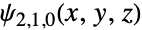
SliceContourPlot3D[(Abs@ψ[{2, 1, 0}, {Sqrt[x^2 + y^2 + z^2], ArcTan[z, Sqrt[x^2 + y^2]], ArcTan[x, y]}])^2, "CenterCutSphere", {x, -5 a0, 5 a0}, {y, -5 a0, 5 a0}, {z, -5 a0, 5 a0}, Contours -> 5, PlotLegends -> Automatic]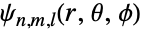
Grid@(Flatten /@ Table[SliceContourPlot3D[(Abs@ψ[{n, l, m}, {Sqrt[x^2 + y^2 + z^2], ArcTan[z, Sqrt[x^2 + y^2]], ArcTan[x, y]}])^2, "CenterCutSphere", {x, -5 a0, 5 a0}, {y, -5 a0, 5 a0}, {z, -5 a0, 5 a0}, Contours -> 5, PlotLabel -> {n, l, m}, Axes -> None, Boxed -> False, ImageSize -> Tiny], {n, 1, 3}, {l, 0, n - 1}, {m, -l, l}])

ElectroStaticPotential[ql_, pl_, r_] := Sum[ (ql[[i]]/Norm[r - pl[[i]]]), {i, Length[ql]}]ElectroStaticPotential[{Subscript[q, 1], Subscript[q, 2]}, {{Subscript[x, 1], Subscript[y, 1], Subscript[z, 1]}, {Subscript[x, 2], Subscript[y, 2], Subscript[z, 2]}}, {x, y, z}]//TraditionalForm

p1 = SliceContourPlot3D[Evaluate[Clip@ElectroStaticPotential[{1, -1}, {{-1, -1, 0}, {1, 1, 0}}, {x, y, z}]], "ZStackedPlanes", {x, -2, 2}, {y, -2, 2}, {z, -2, 2}, ColorFunction -> "Rainbow", PlotLegends -> Automatic, PlotPoints -> 50]p2 = ContourPlot3D[Evaluate[ElectroStaticPotential[{1, -1}, {{-1, -1, 0}, {1, 1, 0}}, {x, y, z}]], {x, -2, 2}, {y, -2, 2}, {z, -2, 2}, Contours -> {-0.3, 0, 0.3}, Mesh -> None, ContourStyle -> Opacity[0.8]]Show[p1, p2]偏微分方程 (3)
使用周期性边界条件(periodic boundary conditions)在两个空间维度中可视化一个非线性的 sine-Gordon 方程,z 轴表示时间:
L = 4;
usol = NDSolveValue[{D[u[t, x, y], t, t] == D[u[t, x, y], x, x] + D[u[t, x, y], y, y] + Sin[u[t, x, y]], u[t, -L, y] == u[t, L, y], u[t, x, -L] == u[t, x, L], u[0, x, y] == Exp[-(x ^ 2 + y ^ 2)], Derivative[1, 0, 0][u][0, x, y] == 0}, u, {t, 0, L / 2}, {x, -L, L}, {y, -L, L}]SliceContourPlot3D[usol[t, x, y], "CenterCutSphere", {x, -L, L}, {y, -L, L}, {t, 0, L / 2}, AxesLabel -> Automatic, PlotLegends -> Automatic]在两个空间维度中可视化 Wolfram 的非线性波动方程,z 轴表示时间:
usol = NDSolveValue[{D[u[t, x, y], t, t] == D[u[t, x, y], x, x] + D[u[t, x, y], y, y] / 2 + (1 - u[t, x, y] ^ 2)(1 + 2u[t, x, y]), u[0, x, y] == E^-(x^2 + y^2), u[t, -5, y] == u[t, 5, y], u[t, x, -5] == u[t, x, 5], u^(1, 0, 0)[0, x, y] == 0}, u, {t, 0, 4}, {x, -5, 5}, {y, -5, 5}]SliceContourPlot3D[usol[t, x, y], "CenterCutSphere", {x, -5, 5}, {y, -5, 5}, {t, 1, 4}, AxesLabel -> Automatic, ColorFunction -> "BrightBands", PlotLegends -> Automatic]可视化三维偏微分方程的解. 在此例中,为一个 Ball 上的泊松方程(Poisson equation)和狄利克雷边界条件(Dirichlet boundary conditions):
usol = NDSolveValue[{Subsuperscript[∇, {x, y, z}, 2]u[x, y, z] == 1, DirichletCondition[u[x, y, z] == x y z, True]}, u, {x, y, z}∈Ball[]]SliceContourPlot3D[usol[x, y, z], "XStackedPlanes", {x, y, z}∈Ball[]]属性和关系 (5)
用 SliceDensityPlot3D 在曲面上绘制连续密度图:
{SliceDensityPlot3D[x ^ 2 + y ^ 2 + z ^ 2, "BackPlanes", {x, -2, 2}, {y, -2, 2}, {z, -2, 2}], SliceContourPlot3D[x ^ 2 + y ^ 2 + z ^ 2, "BackPlanes", {x, -2, 2}, {y, -2, 2}, {z, -2, 2}]}用 ContourPlot3D 来绘制数值为常数的曲面:
{ContourPlot3D[x ^ 2 + y ^ 2 + z ^ 2, {x, -2, 2}, {y, -2, 2}, {z, -2, 2}], SliceContourPlot3D[x ^ 2 + y ^ 2 + z ^ 2, "CenterPlanes", {x, -2, 2}, {y, -2, 2}, {z, -2, 2}, Contours -> 3]}用 DensityPlot3D 来呈现数值的整体可视化:
{DensityPlot3D[x y z, {x, -2, 2}, {y, -2, 2}, {z, -2, 2}], SliceContourPlot3D[x y z, "BackPlanes", {x, -2, 2}, {y, -2, 2}, {z, -2, 2}]}对数据使用 ListSliceContourPlot3D:
data = Table[Sin[x] + y ^ 2 - z ^ 3, {z, -1, 1, 0.1}, {y, -1, 1, 0.1}, {x, -1, 1, 0.1}];{ListSliceContourPlot3D[data, "BackPlanes"], SliceContourPlot3D[Sin[x] + y ^ 2 - z ^ 3, "BackPlanes", {x, -1, 1}, {y, -1, 1}, {z, -1, 1}]}用 ContourPlot 得到二维等高线图:
{ContourPlot[x ^ 2 + y ^ 2, {x, -1, 1}, {y, -1, 1}], SliceContourPlot3D[x ^ 2 + y ^ 2, "BackPlanes", {x, -1, 1}, {y, -1, 1}, {z, -1, 1}]}可能存在的问题 (1)
SliceContourPlot3D[x ^ 2 + y ^ 2 + z ^ 2, "CenterSphere", {x, -1, 1}, {y, -1, 1}, {z, -1, 1}]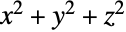
ContourPlot3D[x ^ 2 + y ^ 2 + z ^ 2 == 1, {x, -1, 1}, {y, -1, 1}, {z, -1, 1}]SliceContourPlot3D[x ^ 2 + y ^ 2 + z ^ 2, "CenterPlanes", {x, -1, 1}, {y, -1, 1}, {z, -1, 1}]文本
Wolfram Research (2015),SliceContourPlot3D,Wolfram 语言函数,https://reference.wolfram.com/language/ref/SliceContourPlot3D.html (更新于 2022 年).
CMS
Wolfram 语言. 2015. "SliceContourPlot3D." Wolfram 语言与系统参考资料中心. Wolfram Research. 最新版本 2022. https://reference.wolfram.com/language/ref/SliceContourPlot3D.html.
APA
Wolfram 语言. (2015). SliceContourPlot3D. Wolfram 语言与系统参考资料中心. 追溯自 https://reference.wolfram.com/language/ref/SliceContourPlot3D.html 年