


ListVectorPlot
ListVectorPlot[varr]
generates a vector plot from an array varr of vectors.
ListVectorPlot[{{{x1,y1},{vx1,vy1}},…}]
generates a vector plot from vectors {vxi,vyi} given at specified points {xi,yi}.
ListVectorPlot[{data1,data2,…}]
plots data for several vector fields.
Details and Options
- ListVectorPlot is also known as field plot and direction plot.
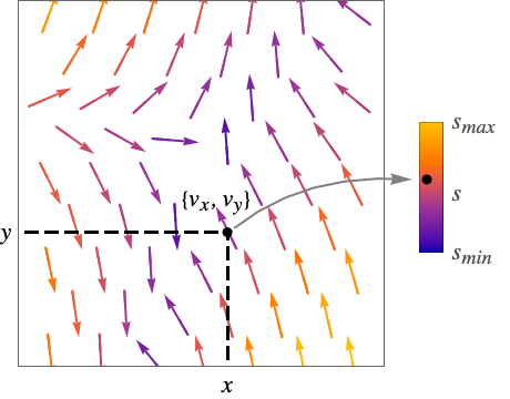
- ListVectorPlot displays a vector field
 by drawing arrows normalized to a fixed length. The arrows are colored by default according to the magnitude
  of the vector field.
 - The plot visualizes the set
 , where
  is the region for which
  is defined.
 - ListVectorPlot interpolates the data into field functions
 .
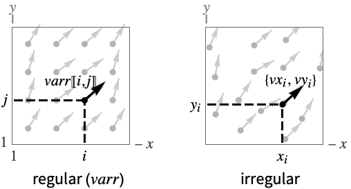
. - For regular data, the vector field
 has value varr〚i,j〛 at
  .
. - For irregular data, the vector field
 has value {vxi,vyi} at
  .
. - ListVectorPlot[varr] arranges successive rows of varr up the page and successive columns across.
- ListVectorPlot by default interpolates the data given and plots vectors for the vector field at a specified grid of positions.
- ListVectorPlot has the same options as Graphics, with the following additions and changes: [List of all options]
-
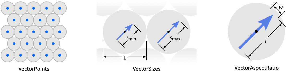
AspectRatio 1 ratio of height to width ClippingStyle Automatic how to display arrows outside the vector range DataRange Automatic the range of x and y values to assume for data Frame True whether to draw a frame around the plot FrameTicks Automatic frame tick marks Method Automatic methods to use for the plot PerformanceGoal $PerformanceGoal aspects of performance to try to optimize PlotLayout Automatic how to position fields PlotLegends None legends for vector fields PlotRange {Full,Full} range of x, y values to include PlotRangePadding Automatic how much to pad the range of values PlotTheme $PlotTheme overall theme for the plot RegionFunction (True&) determine what region to include RegionBoundaryStyle Automatic how to style plot region boundaries RegionFillingStyle Automatic how to style plot region interiors ScalingFunctions None how to scale individual coordinates VectorAspectRatio Automatic width to length ratio for arrows VectorColorFunction Automatic how to color arrows VectorColorFunctionScaling True whether to scale the argument to VectorColorFunction VectorMarkers Automatic shape to use for arrows VectorPoints Automatic the number or placement of arrows VectorRange Automatic range of vector lengths to show VectorScaling None how to scale the sizes of arrows VectorSizes Automatic sizes of displayed arrows VectorStyle Automatic how to draw vectors - The individual arrows are scaled to fit inside bounding circles around each point.
- With the setting VectorPoints->All, ListVectorPlot instead shows vectors associated with the particular vector field data points given.
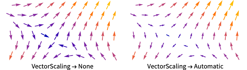
- VectorScaling scales the magnitudes of the vectors into the range of arrow sizes smin to smax given by VectorSizes.
- VectorScaling->Automatic will scale the arrow lengths depending on the vector magnitudes:
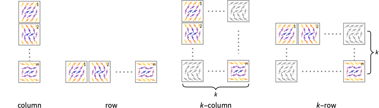
- Possible settings for PlotLayout that show a single group of vectors in multiple plot panels include:
-
"Column" use separate group of vectors in a column of panels "Row" use separate group of vectors in a row of panels {"Column",k},{"Row",k} use k columns or rows {"Column",UpTo[k]},{"Row",UpTo[k]} use at most k columns or rows - The arrow markers given by VectorMarkers are drawn inside a box whose width and length are in the proportion
 specified by VectorAspectRatio.
 - Common markers include:
-

"Segment" line segment aligned in the field direction 
"PinDart" pin dart aligned along the field 
"Dart" dart-shaped marker 
"Drop" drop-shaped marker - VectorColorFunction->None will draw the arrows with the style specified by VectorStyle.
- The arguments supplied to functions in RegionFunction and VectorColorFunction are x, y, vx, vy, Norm[{vx,vy}].
- Possible settings for ScalingFunctions are:
-
{sx,sy} scale x and y axes - Common built-in scaling functions s include:
-
"Log" 
log scale with automatic tick labeling "Log10" 
base-10 log scale with powers of 10 for ticks "SignedLog" 
log-like scale that includes 0 and negative numbers "Reverse" 
reverse the coordinate direction "Infinite" 
infinite scale
List of all options
Examples
open all close allBasic Examples (4)
Plot the vector field interpolated from a specified set of vectors:
ListVectorPlot[Table[{y, -x}, {x, -3, 3, 0.2}, {y, -3, 3, 0.2}]]Include a legend showing the vector magnitudes:
data = Table[{{x, y}, {y, -x}}, {x, -3, 3, 0.2}, {y, -3, 3, 0.2}];ListVectorPlot[data, PlotLegends -> Automatic]Use a drop-shaped marker to represent the vectors:
ListVectorPlot[Table[{x + y, y - x}, {x, -3, 3, 0.2}, {y, -3, 3, 0.2}], VectorMarkers -> "Drop"]Use a multi-panel layout to show multiple vector fields at the same time:
ListVectorPlot[{IconizedObject[«data1»], IconizedObject[«data2»]}, PlotLayout -> "Row"]Scope (16)
Sampling (6)
Plot vectors for a regular collection of vectors, and give a data range for the domain:
ListVectorPlot[Table[{y, -x}, {x, -3, 3, 0.2}, {y, -3, 3, 0.2}], DataRange -> {{-3, 3}, {-3, 3}}]Plot an irregular collection of vectors:
data = Table[{{x, y} = RandomReal[{-3, 3}, {2}], {y, -x}}, {200}];ListVectorPlot[data]Show all of the specified field vectors:
ListVectorPlot[data, VectorPoints -> All]Explicitly set the number of vectors in each direction:
ListVectorPlot[data, VectorPoints -> {4, 7}]Specify a list of points for showing field vectors:
ListVectorPlot[Table[{y, -x}, {x, -3, 3, 0.2}, {y, -3, 3, 0.2}], DataRange -> {{-3, 3}, {-3, 3}}, VectorSizes -> Large, VectorPoints -> RandomReal[{-3, 3}, {300, 2}]]Plot a vector field with vectors placed with specified densities:
data = Table[{y, -x}, {x, -2, 2, 0.2}, {y, -2, 2, 0.2}];Table[ListVectorPlot[data, PlotLabel -> p, VectorPoints -> p], {p, {5, Coarse, Automatic, Fine}}]Plot the vectors that go through a set of seed points:
points = {{-1, -1}, {-1, 1}, {0, 0}, {1, -1}, {1, 1}};
data = Table[{-1 - x ^ 2 + y, 1 + x - y ^ 2}, {x, -2, 2, 0.2}, {y, -2, 2, 0.2}];ListVectorPlot[data, DataRange -> {{-2, 2}, {-2, 2}}, VectorPoints -> points, Epilog -> {Red, PointSize[Medium], Point[points]}]Plot vectors over a specified region:
ListVectorPlot[Table[{{x, y} = RandomReal[{-3, 3}, {2}], {y, -x}}, {200}], RegionFunction -> Function[{x, y, vx, vy, n}, x y < 0]]Presentation (10)
Plot a vector field with arrows scaled according to their magnitudes:
ListVectorPlot[Table[{y, -x}, {x, -3, 3, 0.2}, {y, -3, 3, 0.2}], VectorScaling -> Automatic]Use a single color for the arrows:
ListVectorPlot[Table[{y, -x}, {x, -3, 3, 0.2}, {y, -3, 3, 0.2}], VectorColorFunction -> None]Plot a vector field with arrows of specified size:
data = Table[{x, -y}, {x, -3, 3, 0.2}, {y, -3, 3, 0.2}];Table[ListVectorPlot[data, VectorColorFunction -> "BrightBands", PlotLabel -> s, VectorSizes -> s], {s, {Small, Medium, Large, 0.5}}]Plot a vector field with arrows colored according to the magnitude of the field:
ListVectorPlot[Table[{y, -x}, {x, -3, 3, 0.2}, {y, -3, 3, 0.2}], VectorColorFunction -> "Rainbow"]Set the style for multiple vector fields:
data1 = Table[{-1 - x ^ 2 + y, 1 + x - y ^ 2}, {x, -3, 3, 0.2}, {y, -3, 3, 0.2}];
data2 = Table[{-(1 + x - y ^ 2), -1 - x ^ 2 + y}, {x, -3, 3, 0.2}, {y, -3, 3, 0.2}];ListVectorPlot[{data1, data2}, VectorPoints -> 8, VectorMarkers -> {"Drop", "Dart"}]data = Table[{-1 - x ^ 2 + y, 1 + x - y ^ 2}, {x, -3, 3, 0.2}, {y, -3, 3, 0.2}];ListVectorPlot[data, VectorPoints -> 8, VectorStyle -> Arrowheads[{{0.03, Automatic, Graphics[Circle[]]}}]]Use a named appearance to draw the vectors:
data = Table[{y, -x}, {x, -3, 3, 0.2}, {y, -3, 3, 0.2}];ListVectorPlot[data, VectorMarkers -> "Drop"]ListVectorPlot[data, VectorMarkers -> "Drop", VectorColorFunction -> None, VectorStyle -> Red]data1 = Table[{-1 - x ^ 2 + y, 1 + x - y ^ 2}, {x, -3, 3, 0.2}, {y, -3, 3, 0.2}];
data2 = Table[{-(1 + x - y ^ 2), -1 - x ^ 2 + y}, {x, -3, 3, 0.2}, {y, -3, 3, 0.2}];ListVectorPlot[{data1, data2}, PlotTheme -> "Detailed"]Combine the theme with a specific style for the vectors:
ListVectorPlot[{data1, data2}, PlotTheme -> "Detailed", VectorMarkers -> "Dart"]Show multiple vector fields in separate panels:
ListVectorPlot[{IconizedObject[«field1»], IconizedObject[«field1»]}, PlotLayout -> "Row"]Use a column instead of a row:
ListVectorPlot[{IconizedObject[«field1»], IconizedObject[«field1»]}, PlotLayout -> "Column"]Use a log scale in the y direction:
ListVectorPlot[Table[{y, x + y}, {x, -1, 1, 0.1}, {y, -1, 1, 0.1}], ScalingFunctions -> {None, "Log"}]Options (95)
AspectRatio (3)
By default, ListVectorPlot uses the same width and height:
ListVectorPlot[IconizedObject[«field»]]Use numerical value to specify the height to width ratio:
ListVectorPlot[IconizedObject[«field»], AspectRatio -> 1 / GoldenRatio]AspectRatioAutomatic determines the ratio from the plot ranges:
ListVectorPlot[IconizedObject[«field»], AspectRatio -> Automatic]Axes (4)
By default, ListVectorPlot uses a frame instead of axes:
ListVectorPlot[IconizedObject[«field»]]ListVectorPlot[IconizedObject[«field»], Frame -> False, Axes -> True]Use AxesOrigin to specify where the axes intersect:
ListVectorPlot[IconizedObject[«field»], Frame -> False, Axes -> True, AxesOrigin -> {1, 1}]Turn each axis on individually:
{ListVectorPlot[IconizedObject[«field»], Frame -> False, Axes -> {True, False}], ListVectorPlot[IconizedObject[«field»], Frame -> False, Axes -> {False, True}]}AxesLabel (3)
No axes labels are drawn by default:
ListVectorPlot[IconizedObject[«field»], Frame -> False, Axes -> True]ListVectorPlot[IconizedObject[«field»], Frame -> False, Axes -> True, AxesLabel -> y]ListVectorPlot[IconizedObject[«field»], Frame -> False, Axes -> True, AxesLabel -> {x, y}]AxesOrigin (2)
The position of the axes is determined automatically:
ListVectorPlot[IconizedObject[«field»], Frame -> False, Axes -> True]Specify an explicit origin for the axes:
ListVectorPlot[IconizedObject[«field»], Frame -> False, Axes -> True, AxesOrigin -> {1, 1}]AxesStyle (4)
Change the style for the axes:
ListVectorPlot[IconizedObject[«field»], Frame -> False, Axes -> True, AxesStyle -> Red]Specify the style of each axis:
ListVectorPlot[IconizedObject[«field»], Frame -> False, Axes -> True, AxesStyle -> {Red, Blue}]Use different styles for the ticks and the axes:
ListVectorPlot[IconizedObject[«field»], Frame -> False, Axes -> True, AxesStyle -> Green, TicksStyle -> Red]Use different styles for the labels and the axes:
ListVectorPlot[IconizedObject[«field»], Frame -> False, Axes -> True, AxesStyle -> Green, LabelStyle -> Red]Background (1)
DataRange (1)
By default, the data range is taken to be the index range of the data array:
data = Table[{y, -x}, {x, -3, 3, 0.2}, {y, -3, 3, 0.3}];
Dimensions[data]ListVectorPlot[data]Specify the data range for the domain:
ListVectorPlot[data, DataRange -> {{-3, 3}, {-3, 3}}]EvaluationMonitor (1)
ImageSize (5)
Use named sizes such as Tiny, Small, Medium and Large:
{ListVectorPlot[IconizedObject[«field»], ImageSize -> Tiny], ListVectorPlot[IconizedObject[«field»], ImageSize -> Small]}Specify the width of the plot:
{ListVectorPlot[IconizedObject[«field»], ImageSize -> 150], ListVectorPlot[IconizedObject[«field»], AspectRatio -> 1.5, ImageSize -> 150]}Specify the height of the plot:
{ListVectorPlot[IconizedObject[«field»], ImageSize -> {Automatic, 150}], ListVectorPlot[IconizedObject[«field»], AspectRatio -> 2, ImageSize -> {Automatic, 150}]}Allow the width and height to be up to a certain size:
{ListVectorPlot[IconizedObject[«field»], ImageSize -> UpTo[200]], ListVectorPlot[IconizedObject[«field»], AspectRatio -> 2, ImageSize -> UpTo[200]]}Specify the width and height for a graphic, padding with space if necessary:
ListVectorPlot[IconizedObject[«field»], ImageSize -> {300, 200}, Background -> StandardGray]Setting AspectRatioFull will fill the available space:
ListVectorPlot[IconizedObject[«field»], AspectRatio -> Full, ImageSize -> {300, 200}, Background -> StandardGray]Use maximum sizes for the width and height:
{ListVectorPlot[IconizedObject[«field»], ImageSize -> {UpTo[150], UpTo[100]}], ListVectorPlot[IconizedObject[«field»], AspectRatio -> 2, ImageSize -> {UpTo[150], UpTo[100]}]}PerformanceGoal (2)
Generate a higher-quality plot:
ListVectorPlot[Table[{-1 - x ^ 2 + y, 1 + x - y ^ 2}, {x, -3, 3, 0.2}, {y, -3, 3, 0.2}], PerformanceGoal -> "Quality"]Emphasize performance, possibly at the cost of quality:
ListVectorPlot[Table[{-1 - x ^ 2 + y, 1 + x - y ^ 2}, {x, -3, 3, 0.2}, {y, -3, 3, 0.2}], PerformanceGoal -> "Speed"]PlotLayout (3)
Place each field in a separate panel using shared axes:
ListVectorPlot[{IconizedObject[«x + y»], IconizedObject[«-x + y»]}, ImageSize -> Medium, PlotLayout -> "Column"]Use a row instead of a column:
ListVectorPlot[{IconizedObject[«x + y»], IconizedObject[«-x + y»]}, ImageSize -> Medium, PlotLayout -> "Row"]ListVectorPlot[{IconizedObject[«x + y»], IconizedObject[«-x»], IconizedObject[«y»], IconizedObject[«-x + y»]}, ImageSize -> Medium, PlotLayout -> {"Column", 2}]ListVectorPlot[{IconizedObject[«x + y»], IconizedObject[«-x»], IconizedObject[«y»], IconizedObject[«x»], IconizedObject[«-x + y»], IconizedObject[«0»]}, ImageSize -> Medium, PlotLayout -> {"Column", UpTo[4]}]ListVectorPlot[{IconizedObject[«x + y»], IconizedObject[«-x»], IconizedObject[«y»], IconizedObject[«x»], IconizedObject[«-x + y»], IconizedObject[«0»]}, ImageSize -> Medium, PlotLayout -> {"Column", 4}]PlotLegends (2)
No legends are included by default:
ListVectorPlot[Table[{y, Exp[-x]}, {x, -3, 3, 0.3}, {y, -3, 3, 0.3}]]Include a legend to show the color range of vector norms:
ListVectorPlot[Table[{y, Exp[-x]}, {x, -3, 3, 0.3}, {y, -3, 3, 0.3}], PlotLegends -> Automatic]Add legends with placeholder text:
data1 = Table[{y, -x}, {x, -3, 3, 0.2}, {y, -3, 3, 0.2}];
data2 = Table[{x, y}, {x, -3, 3, 0.2}, {y, -3, 3, 0.2}];ListVectorPlot[{data1, data2}, VectorColorFunction -> None, PlotLegends -> Automatic]Specify labels for the legend:
ListVectorPlot[{data1, data2}, PlotLegends -> {"one", "two"}, VectorColorFunction -> None]Place the legend below the plot:
ListVectorPlot[{data1, data2}, VectorColorFunction -> None, PlotLegends -> Placed[{"one", "two"}, Below]]Control the appearance of the legend:
ListVectorPlot[{data1, data2}, VectorColorFunction -> None, PlotLegends -> SwatchLegend[{"one", "two"}, LegendMarkerSize -> {40, 10}]]PlotRange (7)
The full plot range is used by default:
ListVectorPlot[Table[{-1 - x ^ 2 + y, 1 + x - y ^ 2}, {x, -3, 3, 0.2}, {y, -3, 3, 0.2}], PlotRange -> Full]Specify an explicit limit for both ![]() and
and ![]() ranges:
ranges:
ListVectorPlot[Table[{-1 - x ^ 2 + y, 1 + x - y ^ 2}, {x, -3, 3, 0.2}, {y, -3, 3, 0.2}], DataRange -> {{-3, 3}, {-3, 3}}, PlotRange -> 2]ListVectorPlot[Table[{-1 - x ^ 2 + y, 1 + x - y ^ 2}, {x, -3, 3, 0.2}, {y, -3, 3, 0.2}], DataRange -> {{-3, 3}, {-3, 3}}, PlotRange -> {{-1, 2}, Automatic}]Specify an explicit ![]() minimum range:
minimum range:
ListVectorPlot[Table[{-1 - x ^ 2 + y, 1 + x - y ^ 2}, {x, -3, 3, 0.2}, {y, -3, 3, 0.2}], DataRange -> {{-3, 3}, {-3, 3}}, PlotRange -> {{0, Full}, Automatic}]ListVectorPlot[Table[{-1 - x ^ 2 + y, 1 + x - y ^ 2}, {x, -3, 3, 0.2}, {y, -3, 3, 0.2}], DataRange -> {{-3, 3}, {-3, 3}}, PlotRange -> {Full, {0, 2}}]Specify an explicit ![]() maximum range:
maximum range:
ListVectorPlot[Table[{-1 - x ^ 2 + y, 1 + x - y ^ 2}, {x, -3, 3, 0.2}, {y, -3, 3, 0.2}], DataRange -> {{-3, 3}, {-3, 3}}, PlotRange -> {Full, {Full, 5}}]ListVectorPlot[Table[{-1 - x ^ 2 + y, 1 + x - y ^ 2}, {x, -3, 3, 0.2}, {y, -3, 3, 0.2}], DataRange -> {{-3, 3}, {-3, 3}}, PlotRange -> {{-2, 1.5}, {-1, 2}}]PlotTheme (1)
Use a theme with gridlines, dark background and bold colors:
data = Table[{-1 - x ^ 2 + y, 1 + x - y ^ 2}, {x, -3, 3, 0.2}, {y, -3, 3, 0.2}];ListVectorPlot[data, PlotTheme -> "Marketing"]Change the VectorColorFunction:
ListVectorPlot[data, PlotTheme -> "Marketing", VectorColorFunction -> Hue]RegionBoundaryStyle (5)
Show the region defined by a region function:
ListVectorPlot[Table[{x, y}, {x, -1, 1, 0.1}, {y, -1, 1, 0.1}], RegionFunction -> Function[{x, y}, x + y > 0], DataRange -> {{-1, 1}, {-1, 1}}]The boundaries of full rectangular regions are not shown:
ListVectorPlot[Table[{x, y}, {x, -1, 1, 0.1}, {y, -1, 1, 0.1}]]Use None to not show the boundary:
ListVectorPlot[Table[{x, y}, {x, -1, 1, 0.1}, {y, -1, 1, 0.1}], RegionFunction -> Function[{x, y}, x^2 + y^2 < 1], DataRange -> {{-1, 1}, {-1, 1}}, RegionBoundaryStyle -> None]Omit the interior filling as well:
ListVectorPlot[Table[{x, y}, {x, -1, 1, 0.1}, {y, -1, 1, 0.1}], RegionFunction -> Function[{x, y}, x^2 + y^2 < 1], DataRange -> {{-1, 1}, {-1, 1}}, RegionBoundaryStyle -> None, RegionFillingStyle -> None]Specify a style for the boundary:
ListVectorPlot[Table[{x, y}, {x, -1, 1, 0.1}, {y, -1, 1, 0.1}], RegionFunction -> Function[{x, y}, x^2 + y^2 < 1], DataRange -> {{-1, 1}, {-1, 1}}, RegionBoundaryStyle -> Red]Specify a style for full rectangular regions:
ListVectorPlot[Table[{x, y}, {x, -1, 1, 0.1}, {y, -1, 1, 0.1}], RegionBoundaryStyle -> Red]RegionFillingStyle (5)
Show the region defined by a region function:
ListVectorPlot[Table[{x, y}, {x, -1, 1, 0.1}, {y, -1, 1, 0.1}], RegionFunction -> Function[{x, y}, x + y > 0], DataRange -> {{-1, 1}, {-1, 1}}]The interior of full rectangular regions are not shown:
ListVectorPlot[Table[{x, y}, {x, -1, 1, 0.1}, {y, -1, 1, 0.1}]]Use None to not show the interior filling:
ListVectorPlot[Table[{x, y}, {x, -1, 1, 0.1}, {y, -1, 1, 0.1}], RegionFunction -> Function[{x, y}, x^2 + y^2 < 1], DataRange -> {{-1, 1}, {-1, 1}}, RegionFillingStyle -> None]Omit the boundary curve as well:
ListVectorPlot[Table[{x, y}, {x, -1, 1, 0.1}, {y, -1, 1, 0.1}], RegionFunction -> Function[{x, y}, x^2 + y^2 < 1], DataRange -> {{-1, 1}, {-1, 1}}, RegionBoundaryStyle -> None, RegionFillingStyle -> None]Specify a style for the interior filling:
ListVectorPlot[Table[{x, y}, {x, -1, 1, 0.1}, {y, -1, 1, 0.1}], RegionFunction -> Function[{x, y}, x^2 + y^2 < 1], DataRange -> {{-1, 1}, {-1, 1}}, RegionFillingStyle -> Gray]Specify a style for full rectangular region:
ListVectorPlot[Table[{x, y}, {x, -1, 1, 0.1}, {y, -1, 1, 0.1}], RegionFillingStyle -> Gray]RegionFunction (3)
Plot vectors only over certain quadrants:
data = Table[{-1 - x ^ 2 + y, 1 + x - y ^ 2}, {x, -3, 3, 0.2}, {y, -3, 3, 0.2}];ListVectorPlot[data, DataRange -> {{-3, 3}, {-3, 3}}, RegionFunction -> Function[{x, y, vx, vy, n}, x y < 0]]Plot vectors only over regions where the field magnitude is above a given threshold:
data = Table[{-1 - x ^ 2 + y, 1 + x - y ^ 2}, {x, -3, 3, 0.2}, {y, -3, 3, 0.2}];ListVectorPlot[data, DataRange -> {{-3, 3}, {-3, 3}}, RegionFunction -> Function[{x, y, vx, vy, n}, n > 6]]Use any logical combination of conditions:
data = Table[{-1 - x ^ 2 + y, 1 + x - y ^ 2}, {x, -3, 3, 0.2}, {y, -3, 3, 0.2}];ListVectorPlot[data, DataRange -> {{-3, 3}, {-3, 3}}, RegionFunction -> Function[{x, y, vx, vy, n}, 4 < n < 9 || 0 < n < 2]]ScalingFunctions (3)
By default, linear scales are used:
ListVectorPlot[Table[{y, x - y}, {x, -1, 1, 0.1}, {y, -1, 1, 0.1}]]Use a log scale in the y direction:
ListVectorPlot[Table[{y, x - y}, {x, -1, 1, 0.1}, {y, -1, 1, 0.1}], ScalingFunctions -> {None, "Log"}]Reverse the direction of the y direction:
ListVectorPlot[Table[{y, x - y}, {x, -1, 1, 0.1}, {y, -1, 1, 0.1}], ScalingFunctions -> {None, "Reverse"}]VectorColorFunction (4)
Color the vectors according to their norms:
data = Table[{y, -x}, {x, -3, 3, 0.2}, {y, -3, 3, 0.2}];ListVectorPlot[data, VectorColorFunction -> Hue]Use any named color gradient from ColorData:
data = Table[{y, -x}, {x, -3, 3, 0.2}, {y, -3, 3, 0.2}];ListVectorPlot[data, VectorColorFunction -> "Rainbow"]Color the vectors according to their ![]() values:
values:
data = Table[{y, -x}, {x, -3, 3, 0.2}, {y, -3, 3, 0.2}];ListVectorPlot[data, VectorColorFunction -> Function[{x, y, vx, vy, n}, ColorData["ThermometerColors"][x]]]Use VectorColorFunctionScaling->False to get unscaled values:
data = Table[{y, -x}, {x, -3, 3, 0.2}, {y, -3, 3, 0.2}];ListVectorPlot[data, VectorColorFunction -> Function[{x, y, vx, vy, n}, ColorData[22][Round[n]]], VectorColorFunctionScaling -> False]VectorColorFunctionScaling (4)
By default, scaled values are used:
ListVectorPlot[Table[{y, -x}, {x, -3, 3, 0.2}, {y, -3, 3, 0.2}], VectorColorFunction -> Hue]Use VectorColorFunctionScaling->False to get unscaled values:
data = Table[{y, -x}, {x, -3, 3, 0.2}, {y, -3, 3, 0.2}];ListVectorPlot[data, VectorColorFunction -> Function[{x, y, vx, vy, n}, ColorData[22][Round[n]]], VectorColorFunctionScaling -> False]Use unscaled coordinates in the ![]() direction and scaled coordinates in the
direction and scaled coordinates in the ![]() direction:
direction:
data = Table[{y, -x}, {x, -3, 3, 0.2}, {y, -3, 3, 0.2}];ListVectorPlot[data, VectorColorFunction -> Function[{x, y, vx, vy, n}, Hue[x, y, 1]], VectorColorFunctionScaling -> {False, True},
DataRange -> {{0, 1}, {0, 1}}]Explicitly specify the scaling for each color function argument:
data = Table[{y, -x}, {x, -3, 3, 0.2}, {y, -3, 3, 0.2}];ListVectorPlot[data, VectorColorFunction -> Function[{x, y, vx, vy, n}, Hue[n, y, 1]], VectorColorFunctionScaling -> {True, True, True, True, False}]VectorMarkers (9)
Vectors are drawn as arrows by default:
data = Table[{y, -x}, {x, -3, 3, 0.2}, {y, -3, 3, 0.2}];ListVectorPlot[data]Use a named appearance to draw the vectors:
data = Table[{y, -x}, {x, -3, 3, 0.2}, {y, -3, 3, 0.2}];ListVectorPlot[data, VectorMarkers -> "Drop"]Use different markers for different vector fields:
data1 = Table[{{x, y}, {y, -x}}, {x, -5, 5}, {y, -5, 5}];
data2 = Table[{{x, y}, {x, y}}, {x, -5, 5}, {y, -5, 5}];ListVectorPlot[{data1, data2}, VectorMarkers -> {"Drop", "Dart"}]By default, markers are centered on vector points:
data = Table[{{x, y}, {y, -x}}, {x, -5, 5}, {y, -5, 5}];pts = Tuples[Range[-5, 5], 2];ListVectorPlot[data, VectorMarkers -> "Arrow", VectorPoints -> pts, Epilog -> {Red, Point[pts]}]Start the vectors at the points:
ListVectorPlot[data, VectorMarkers -> Placed["Arrow", "Start"], VectorPoints -> pts, Epilog -> {Red, Point[pts]}]End the vectors at the points:
ListVectorPlot[data, VectorMarkers -> Placed["Arrow", "End"], VectorPoints -> pts, Epilog -> {Red, Point[pts]}]data = Table[{-1 - x ^ 2 + y, 1 + x - y ^ 2}, {x, -3, 3, 0.2}, {y, -3, 3, 0.2}];Table[ListVectorPlot[data, VectorPoints -> 8, PlotLabel -> s, VectorMarkers -> s], {s, {"Arrow", "DotArrow", "ArrowArrow"}}]data = Table[{-1 - x ^ 2 + y, 1 + x - y ^ 2}, {x, -3, 3, 0.2}, {y, -3, 3, 0.2}];Table[ListVectorPlot[data, VectorPoints -> 10, PlotLabel -> s, VectorStyle -> s], {s, {"Circle", "Disk", "CircleArrow"}}]data = Table[{-1 - x ^ 2 + y, 1 + x - y ^ 2}, {x, -3, 3, 0.2}, {y, -3, 3, 0.2}];Table[ListVectorPlot[data, VectorPoints -> 8, PlotLabel -> s, VectorStyle -> s], {s, {"Dart", "PinDart", "DoubleDart"}}]data = Table[{-1 - x ^ 2 + y, 1 + x - y ^ 2}, {x, -3, 3, 0.2}, {y, -3, 3, 0.2}];Table[ListVectorPlot[data, VectorPoints -> 8, PlotLabel -> s, VectorStyle -> s], {s, {"BarDot", "Dot", "DotArrow", "DotDot"}}]data = Table[{-1 - x ^ 2 + y, 1 + x - y ^ 2}, {x, -3, 3, 0.2}, {y, -3, 3, 0.2}];Table[ListVectorPlot[data, VectorPoints -> 8, PlotLabel -> s, VectorStyle -> s], {s, {"Drop", "Pointer", "BackwardPointer", "Toothpick"}}]VectorPoints (8)
Use automatically determined vector points:
ListVectorPlot[Table[{y, -x}, {x, -1, 1, 0.2}, {y, -1, 1, 0.2}], VectorPoints -> Automatic]Show all of the specified field vectors:
ListVectorPlot[Table[{y, -x}, {x, -1, 1, 0.2}, {y, -1, 1, 0.2}], VectorPoints -> All]Use symbolic names to specify the set of field vectors:
data = Table[{y, -x}, {x, -3, 3, 0.2}, {y, -3, 3, 0.2}];Table[ListVectorPlot[data, PlotLabel -> k, VectorPoints -> k], {k, {Fine, Coarse}}]Create a regular grid of field vectors with the same number of arrows for ![]() and
and ![]() :
:
ListVectorPlot[Table[{y, -x}, {x, -3, 3, 0.2}, {y, -3, 3, 0.2}], VectorPoints -> 5]Create a regular grid of field vectors with a different number of arrows for ![]() and
and ![]() :
:
ListVectorPlot[Table[{y, -x}, {x, -3, 3, 0.2}, {y, -3, 3, 0.2}], VectorPoints -> {4, 7}]Specify a list of points for showing field vectors:
data = Table[{-1 - x ^ 2 + y, 1 + x - y ^ 2}, {x, -3, 3, 0.2}, {y, -3, 3, 0.2}];ListVectorPlot[data, DataRange -> {{-3, 3}, {-3, 3}}, VectorPoints -> RandomReal[{-3, 3}, {300, 2}], VectorSizes -> Large]Use a different number of field vectors on a hexagonal grid:
data = Table[{y ^ 2, x ^ 2 - y ^ 2}, {x, -3, 3, 0.2}, {y, -3, 3, 0.2}];Table[ListVectorPlot[data, PlotLabel -> n, VectorPoints -> n, VectorSizes -> Medium], {n, 5, 20, 5}]The location for vectors is given in the middle of the drawn vector:
data = Table[{-1 - x ^ 2 + y, 1 + x - y ^ 2}, {x, -2, 2, 0.2}, {y, -2, 2, 0.2}];
points = {{-1, -1}, {-1, 1}, {0, 0}, {1, -1}, {1, 1}};ListVectorPlot[data, DataRange -> {{-2, 2}, {-2, 2}}, VectorPoints -> points, VectorSizes -> 1, Epilog -> {Red, PointSize[Medium], Point[points]}]VectorRange (4)
The clipping of vectors with very small or very large magnitudes is done automatically:
ListVectorPlot[Table[({x, y}/Norm[{x, y}]^3), {x, -3, 3, 0.35}, {y, -3, 3, 0.35}], VectorRange -> Automatic]Specify the range of vector norms:
ListVectorPlot[Table[({x, y}/Norm[{x, y}]^3), {x, -3, 3, 0.35}, {y, -3, 3, 0.35}], VectorRange -> {0.1, 2}]ListVectorPlot[Table[({x, y}/Norm[{x, y}]^3), {x, -3, 3, 0.35}, {y, -3, 3, 0.35}], VectorRange -> {0.1, 2}, ClippingStyle -> None]ListVectorPlot[Table[({x, y}/Norm[{x, y}]^3), {x, -3, 3, 0.35}, {y, -3, 3, 0.35}], VectorRange -> All]VectorScaling (2)
Use automatically determined vector scales:
ListVectorPlot[Table[{y, -x}, {x, -3, 3, 0.5}, {y, -3, 3, 0.5}], VectorScaling -> Automatic]With the vector scaling function set to None, all vectors have the same size:
ListVectorPlot[Table[{y, -x}, {x, -3, 3, 0.5}, {y, -3, 3, 0.5}], VectorScaling -> None]VectorSizes (2)
The size of the displayed vector is determined automatically:
ListVectorPlot[Table[{y - x(1 - x^2 - y^2)^2, -x - y(1 - x^2 - y^2)^2}, {x, -3, 3, 0.1}, {y, -3, 3, 0.1}], VectorScaling -> Automatic, VectorSizes -> Automatic]Specify the range of arrow lengths:
ListVectorPlot[Table[{y - x(1 - x^2 - y^2)^2, -x - y(1 - x^2 - y^2)^2}, {x, -3, 3, 0.1}, {y, -3, 3, 0.1}], VectorScaling -> Automatic, VectorSizes -> {0, 1}]VectorStyle (7)
VectorColorFunction has precedence over VectorStyle for colors:
ListVectorPlot[Table[{-1 - x ^ 2 + y, 1 + x - y ^ 2}, {x, -3, 3, 0.2}, {y, -3, 3, 0.2}], VectorStyle -> Red]Use VectorColorFunctionNone to style the displayed vectors with VectorStyle:
ListVectorPlot[Table[{-1 - x ^ 2 + y, 1 + x - y ^ 2}, {x, -3, 3, 0.2}, {y, -3, 3, 0.2}], VectorStyle -> Red, VectorColorFunction -> None]Set the style for multiple vector fields:
data1 = Table[{-1 - x ^ 2 + y, 1 + x - y ^ 2}, {x, -3, 3, 0.2}, {y, -3, 3, 0.2}];
data2 = Table[{-(1 + x - y ^ 2), -1 - x ^ 2 + y}, {x, -3, 3, 0.2}, {y, -3, 3, 0.2}];ListVectorPlot[{data1, data2}, VectorPoints -> 8, VectorStyle -> {Red, Blue}, VectorColorFunction -> None]Use Arrowheads to specify an explicit style of the arrowheads:
data = Table[{x, y}, {x, -1, 1, 0.2}, {y, -1, 1, 0.2}];ListVectorPlot[data, VectorPoints -> 8, PlotRange -> All, VectorStyle -> Arrowheads[{{0.03, Automatic, Graphics[Circle[]]}}]]Specify both arrow tail and head:
data = Table[{x, y}, {x, -1, 1, 0.2}, {y, -1, 1, 0.2}];ListVectorPlot[data, VectorPoints -> 8, PlotRange -> All, VectorStyle -> Arrowheads[{{0.03, Automatic, Graphics[Rectangle[{-0.5, -0.5}, {0.5, 0.5}]]}, {0.03, Automatic, Graphics[Circle[]]}}]]Graphics primitives without Arrowheads are scaled based on the VectorSizes:
data = Table[{x, y}, {x, -1, 1, 0.2}, {y, -1, 1, 0.2}];ListVectorPlot[data, VectorPoints -> 8, PlotRange -> All, VectorStyle -> Graphics[Circle[]], VectorSizes -> {0.5, 0.9}]Change the scaling using the VectorSizes option:
data = Table[{x, y}, {x, -1, 1, 0.2}, {y, -1, 1, 0.2}];ListVectorPlot[data, VectorPoints -> 8, PlotRange -> All, VectorStyle -> Graphics[Circle[]], VectorSizes -> {0.2, 0.4}]Applications (3)
data = Table[Evaluate@{D[Sin[x y], {y}], -D[Sin[x y], {x}]}, {x, 0, 2Pi}, {y, 0, 2Pi}];ListVectorPlot[data]Visualize the first horizontal and vertical Gaussian derivatives of an image:
image = ColorConvert[Rasterize[π, ImageSize -> 40, RasterSize -> 40], "Grayscale"]{dx, dy} = Table[ImageAdjust@GaussianFilter[image, {6, 2}, δ], {δ, {{1, 0}, {0, 1}}}]Combine the vertical and horizontal Gaussian derivatives:
data = Reverse /@ Transpose[2ImageData /@ {dx, dy} - 1, {3, 2, 1}];ListVectorPlot[data, VectorPoints -> 30]Characterize linear planar systems interactively:
Manipulate[Row[{Text["m"] == MatrixForm[m], ListVectorPlot[Table[Evaluate[m.{x, y}], {x, -1, 1}, {y, -1, 1}], VectorSizes -> 1, VectorColorFunction -> "Rainbow", ImageSize -> Small]}], {{m, (|   |   |
| - | - |
| 1 | 0 |
| 0 | 2 |)}, {(|   |   |
| - | - |
| 1 | 0 |
| 0 | 2 |) -> "Nodal source", (|   |   |
| - | - |
| 1 | 1 |
| 0 | 1 |) -> "Degenerate source", (|    |   |
| -- | - |
| 0  | 1 |
| -1 | 1 |) -> "Spiral source", (|    |    |
| -- | -- |
| -1 | 0  |
| 0  | -2 |) -> "Nodal sink", (|    |    |
| -- | -- |
| -1 | 1  |
| 0  | -1 |) -> "Degenerate sink", (|    |    |
| -- | -- |
| 0  | 1  |
| -1 | -1 |) -> "Spiral sink", (|    |   |
| -- | - |
| 0  | 1 |
| -1 | 0 |) -> "Center", (|   |    |
| - | -- |
| 1 | 0  |
| 0 | -2 |) -> "Saddle"}}]
Properties & Relations (15)
Use VectorPlot to plot functions:
VectorPlot[{-1 - x ^ 2 + y, 1 + x - y ^ 2}, {x, -3, 3}, {y, -3, 3}]Use StreamPlot to plot streams instead of vectors:
StreamPlot[{-1 - x ^ 2 + y, 1 + x - y ^ 2}, {x, -3, 3}, {y, -3, 3}]Use ListStreamPlot to plot data with streamlines instead of vectors:
ListStreamPlot[Table[{-1 - x ^ 2 + y, 1 + x - y ^ 2}, {x, -3, 3, 0.2}, {y, -3, 3, 0.2}]]Use VectorDensityPlot to add a density plot of a scalar field:
VectorDensityPlot[{-1 - x ^ 2 + y, 1 + x - y ^ 2}, {x, -3, 3}, {y, -3, 3}]Use StreamDensityPlot to use streams instead of vectors:
StreamDensityPlot[{-1 - x ^ 2 + y, 1 + x - y ^ 2}, {x, -3, 3}, {y, -3, 3}]Use ListVectorDensityPlot for plotting data with a density plot of the scalar field:
data = Table[{{x, y} = RandomReal[{-1.5, 1.5}, {2}], {{y, x - x ^ 3}, Abs[x + y]}}, {300}];ListVectorDensityPlot[data]Use ListStreamDensityPlot to plot streams instead of vectors:
ListStreamDensityPlot[data]Use ListLineIntegralConvolutionPlot to plot the line integral convolution of vector field data:
data = Table[{-1 - x ^ 2 + y, 1 + x - y ^ 2}, {x, -3, 3, .2}, {y, -3, 3, .2}];ListLineIntegralConvolutionPlot[data]Use VectorDisplacementPlot to visualize the effect of a displacement vector field on a specified region:
VectorDisplacementPlot[{-1 - x ^ 2 + y, 1 + x - y ^ 2}, {x, y}∈Annulus[], VectorPoints -> Automatic]Use ListVectorDisplacementPlot to visualize the effect of displacement field data on a region:
data = Table[{{x, y}, {x + y, 1 + x - y}}, {x, -3, 3, 0.2}, {y, -3, 3, 0.2}];ListVectorDisplacementPlot[data, Polygon[{{3, 3}, {0, 1}, {-3, 3}, {-3, -3}, {0, -1}, {3, -3}}], VectorPoints -> Automatic]Use VectorPlot3D and StreamPlot3D to visualize 3D vector fields:
{VectorPlot3D[{z, x, x + y}, {x, -1, 1}, {y, -1, 1}, {z, -1, 1}], StreamPlot3D[{z, x, x + y}, {x, -1, 1}, {y, -1, 1}, {z, -1, 1}]}Use ListVectorPlot3D and ListStreamPlot3D to visualize 3D vector field data:
data = Table[{z, -x, y}, {x, -1, 1, .1}, {y, -1, 1, .1}, {z, -1, 1, .1}];{ListVectorPlot3D[data], ListStreamPlot3D[data]}Plot vectors on surfaces with SliceVectorPlot3D:
SliceVectorPlot3D[{-y, x, z}, Sphere[], {x, -1, 1}, {y, -1, 1}, {z, -1, 1}]Plot data vectors on surfaces with ListSliceVectorPlot3D:
ListSliceVectorPlot3D[Table[{-y, x, z}, {x, -1, 1, .1}, {y, -1, 1, .1}, {z, -1, 1, .1}], Sphere[], DataRange -> {{-1, 1}, {-1, 1}, {-1, 1}}]Plot complex functions as a vector field with ComplexVectorPlot:
ComplexVectorPlot[z + 1 / z, {z, 2}]Plot streams instead of vectors with ComplexStreamPlot:
ComplexStreamPlot[z^2 + 1, {z, 2}]Use VectorDisplacementPlot3D to visualize the effect of a displacement vector field on a specified 3D region:
VectorDisplacementPlot3D[{-y, x, x + z}, {x, -2, 2}, {y, -2, 2}, {z, -2, 2}, VectorPoints -> "Boundary"]Use ListVectorDisplacementPlot3D to visualize the effect of a 3D displacement vector field based on data:
data = Table[{{x, y, z}, {-y, x, x + z}}, {x, -2, 2}, {y, -2, 2}, {z, -2, 2}];ListVectorDisplacementPlot3D[data, VectorPoints -> "Boundary"]Use GeoVectorPlot to plot vectors on a map:
GeoVectorPlot[GeoVector[GeoPosition[{{-54.79801473961214, -111.85053058521567},
    {-65.56940402358214, 162.89657500795147}, {-81.67990688759895, -93.36222177594851},
    {7.785750774919734, 95.44840765141487}, {-6.86571958448036, -40.946398330539864},
    { ... 904, "AngularDegrees"]},
   {0.9366099079317551, Quantity[357.70482317743733, "AngularDegrees"]},
   {0.8256817194791912, Quantity[242.07227508889662, "AngularDegrees"]},
   {0.2661401145642981, Quantity[152.90003252279325, "AngularDegrees"]}}]]
Use GeoStreamPlot to use streams instead of vectors:
GeoStreamPlot[GeoVector[GeoPosition[{{-54.79801473961214, -111.85053058521567},
    {-65.56940402358214, 162.89657500795147}, {-81.67990688759895, -93.36222177594851},
    {7.785750774919734, 95.44840765141487}, {-6.86571958448036, -40.946398330539864},
    { ... 904, "AngularDegrees"]},
   {0.9366099079317551, Quantity[357.70482317743733, "AngularDegrees"]},
   {0.8256817194791912, Quantity[242.07227508889662, "AngularDegrees"]},
{0.2661401145642981, Quantity[152.90003252279325, "AngularDegrees"]}}]]Text
Wolfram Research (2008), ListVectorPlot, Wolfram Language function, https://reference.wolfram.com/language/ref/ListVectorPlot.html (updated 2022).
CMS
Wolfram Language. 2008. "ListVectorPlot." Wolfram Language & System Documentation Center. Wolfram Research. Last Modified 2022. https://reference.wolfram.com/language/ref/ListVectorPlot.html.
APA
Wolfram Language. (2008). ListVectorPlot. Wolfram Language & System Documentation Center. Retrieved from https://reference.wolfram.com/language/ref/ListVectorPlot.html